Actuarial Science · Level 201
Actuarial Science 201 — Becoming an Actuary
Loss models, chain-ladder reserving, stress tests and a board-level consulting memo.
Actuarial Science · Level 201
Actuarial Science 201 — Becoming an Actuary
Loss models, chain-ladder reserving, stress tests and a board-level consulting memo.
Actuarial Science 201 — Becoming an Actuary
Prerequisite: Actuarial Science 101.
This course assumes you already completed the Horizon Risk Consulting taster week: you can use VS Code, Jupyter, Python, pandas and matplotlib, and you have an
actuarial101project folder with motor insurance data from Dr. Sarah Okonkwo's team.
You return to Horizon Risk Consulting, a London consultancy that advises insurers, pension schemes and public-sector clients on risk. Your manager is Dr. Sarah Okonkwo, a Fellow of the Institute and Faculty of Actuaries (IFoA) who leads the general insurance practice.
In Actuarial Science 101 you explored what actuaries do, measured claim frequency and severity, built a simple premium calculator and touched flood risk. In this course you go deeper — the kind of work a graduate trainee does in the first year after university, before the professional exam grind fully takes over.
Over five modules you will:
- Fit a loss model — Poisson claim counts plus a severity distribution.
- Price motor policies using driver-age segmentation.
- Estimate IBNR reserves with a chain-ladder run-off triangle.
- Stress-test the portfolio for a climate-related flood scenario.
- Write a consulting memo to the board tying the threads together.
Sample student outputs: Worked examples. Your charts should look broadly similar (frequency, relativities, IBNR, flood stress) — not identical.
The mindset to keep throughout:
frequency → severity → premium → reserve → capital → decision
Before you start — open your actuarial101 folder
In 101 you created a project folder called actuarial101 inside your coding
directory. Open it now.
You should already have:
These two CSV files came from Modules 2 and 3 in 101:
| File | What it contains |
|---|---|
motor_policies.csv |
One row per policy-year: driver age and claim count |
motor_claims.csv |
One row per individual claim: claim amount in pounds |
If either file is missing (for example, you skipped ahead to 201), run the setup cell below once in a new notebook to recreate the teaching dataset. The numbers are synthetic but realistic for UK motor insurance.
Open VS Code. Choose File → Open Folder and open actuarial101.
Create two new subfolders for this course if they are not there yet:
Install anything you have not installed yet:
pip install pandas numpy matplotlib jupyter ipykernelQuick check — are your 101 files present?
Create notebooks/00_check_data.ipynb and run:
Question
Do the motor files from 101 load correctly?
Code
import pandas as pd
from pathlib import Path

data_dir = Path("../data")

for name in ["motor_policies.csv", "motor_claims.csv"]:
    path = data_dir / name
    print(name, "exists:" if path.exists() else "MISSING — run recovery cell below")
    if path.exists():
        print(pd.read_csv(path).head(2), "\n")
If both files exist, delete this notebook and start Module 1.
Recovery — recreate 101 teaching data
Run this only if a file is missing.
Code
import numpy as np
import pandas as pd
from pathlib import Path

rng = np.random.default_rng(42)
data_dir = Path("../data")
data_dir.mkdir(parents=True, exist_ok=True)

# --- motor_policies.csv (frequency side) ---
n_policies = 2000
ages = rng.integers(18, 75, size=n_policies)
# Poisson frequencies with age effect (younger drivers claim more often)
lam = np.clip(0.08 + (30 - np.abs(ages - 30)) * 0.004, 0.03, 0.25)
claim_counts = rng.poisson(lam)

policies = pd.DataFrame({
    "policy_id": [f"P{i:04d}" for i in range(1, n_policies + 1)],
    "policy_year": 2024,
    "driver_age": ages,
    "claim_count": claim_counts,
})
policies.to_csv(data_dir / "motor_policies.csv", index=False)

# --- motor_claims.csv (severity side) ---
rows = []
claim_id = 1
for _, row in policies.iterrows():
    for _ in range(int(row["claim_count"])):
        # Lognormal-ish severities: most small, occasional large
        amount = float(rng.lognormal(mean=7.5, sigma=0.9))
        rows.append({
            "claim_id": f"C{claim_id:05d}",
            "policy_id": row["policy_id"],
            "claim_amount": round(amount, 2),
        })
        claim_id += 1

claims = pd.DataFrame(rows)
claims.to_csv(data_dir / "motor_claims.csv", index=False)

print(policies.shape, claims.shape)
policies["claim_count"].mean(), claims["claim_amount"].mean()
What the code does
We simulate 2,000 policy-years with Poisson claim counts that depend on driver age, then generate individual claim amounts from a skewed distribution. This is the same structure Dr. Okonkwo's team used in 101 — frequency and severity are modelled separately, then combined.
Tools
- VS Code
- Jupyter Notebook
- Python
- pandas
- numpy
- matplotlib
Module 1 — Risk Modelling
Manager email
From: Dr. Sarah Okonkwo
Subject: Build our motor loss model — frequency and severityWelcome back. In 101 you looked at claim counts and claim sizes separately. Now I need a proper loss model for our motor portfolio.
Use
motor_policies.csvfor frequency (how many claims per policy-year) andmotor_claims.csvfor severity (how large each claim is).Deliverables:
- Estimate the average claim frequency (Poisson rate λ).
- Describe the severity distribution — mean, median, and a histogram.
- Simulate total annual losses for 1,000 identical policy-years and show the spread.
- One paragraph: what is the expected total loss per policy-year?
Save charts to
outputs/charts/. Write your paragraph in the notebook.— Sarah
Why this matters
Insurers do not know in advance how many claims they will pay or how large each will be. Actuaries split the problem:
- Frequency — how often claims happen (often modelled as Poisson).
- Severity — how much each claim costs (often right-skewed: many small repairs, a few large write-offs).
The pure premium (expected loss cost) combines both:
where is claim count and is claim size. Professional models add correlation, inflation and cover limits — but this product is the foundation every actuarial student learns.
What you'll learn
- Estimate a Poisson rate from data
- Summarise a skewed severity distribution
- Simulate compound losses (count × size)
- Interpret expected value under uncertainty
Step 1 — Create the notebook
notebooks/module1_risk_modelling.ipynb
Section 1 — Load the 101 motor files
Question
Are frequency and severity in separate tables?
Code
import pandas as pd
import numpy as np
import matplotlib.pyplot as plt

policies = pd.read_csv("../data/motor_policies.csv")
claims = pd.read_csv("../data/motor_claims.csv")

policies.head(), claims.head()
What the code does
motor_policies.csv holds one row per policy-year with a claim count.
motor_claims.csv holds one row per individual claim with an amount.
This mirrors real insurer data warehouses.
Section 2 — Estimate Poisson frequency
Question
What is the average number of claims per policy-year?
Code
lambda_hat = policies["claim_count"].mean()
zero_claim_pct = (policies["claim_count"] == 0).mean()

lambda_hat, zero_claim_pct
What the code does
The sample mean of claim counts is our estimate of λ (lambda), the Poisson rate parameter. Many policy-years have zero claims — that is normal for low-frequency lines like motor.
Under a Poisson model, the probability of zero claims is .
Compare zero_claim_pct to np.exp(-lambda_hat) in a markdown cell — are they
close?
Section 3 — Plot the frequency distribution
Question
Does the shape look Poisson-like?
Code
freq_counts = policies["claim_count"].value_counts().sort_index()

plt.figure(figsize=(7, 4))
plt.bar(freq_counts.index, freq_counts.values, color="steelblue")
plt.xlabel("Claims per policy-year")
plt.ylabel("Number of policies")
plt.title("Observed claim frequency")
plt.savefig("../outputs/charts/module1_frequency.png", dpi=150)
plt.show()
What the code does
Most policies sit at 0 or 1 claims. A few have 2 or more. Poisson models this "mostly zeros, occasionally more" pattern with a single parameter.
Section 4 — Severity summary
Question
How large are individual claims?
Code
severity = claims["claim_amount"]

summary = pd.Series({
    "count": len(severity),
    "mean": severity.mean(),
    "median": severity.median(),
    "max": severity.max(),
    "std": severity.std(),
})
summary
What the code does
For skewed insurance data, the mean exceeds the median — a few large claims pull the average up. Actuaries always report both.
Section 5 — Severity histogram
Question
What does the right tail look like?
Code
plt.figure(figsize=(7, 4))
plt.hist(severity, bins=40, color="coral", edgecolor="white")
plt.xlabel("Claim amount (£)")
plt.ylabel("Count")
plt.title("Claim severity distribution")
plt.savefig("../outputs/charts/module1_severity.png", dpi=150)
plt.show()
What the code does
The histogram should be strongly right-skewed. In practice actuaries often fit Gamma, lognormal or Generalised Pareto distributions to the tail. Here we use the empirical distribution for simulation.
Section 6 — Pure premium (frequency × severity)
Question
What is the expected loss per policy-year?
Code
mean_severity = severity.mean()
pure_premium = lambda_hat * mean_severity

pure_premium
What the code does
If each policy generates λ claims on average and each claim costs £E[X] on average, expected total cost per policy is the product. This is the actuarial pure premium before expenses and profit.
Write a markdown cell explaining this number in plain English (two to three sentences) as if Sarah asked a non-actuary on the team.
Section 7 — Simulate total losses
Question
What range of outcomes could one policy-year produce?
Code
rng = np.random.default_rng(2024)
n_sim = 1000

# Poisson count, then sum that many random severities (with replacement)
sim_totals = []
for _ in range(n_sim):
    n_claims = rng.poisson(lambda_hat)
    if n_claims == 0:
        sim_totals.append(0.0)
    else:
        sim_totals.append(rng.choice(severity.values, size=n_claims).sum())

sim_totals = np.array(sim_totals)
sim_totals.mean(), np.percentile(sim_totals, 95)
What the code does
Each simulation draw: sample a claim count from Poisson(λ), then sample that many severities from the historical claims. Sum them. Repeat 1,000 times.
The mean of sim_totals should be near pure_premium. The 95th percentile
shows a bad but not impossible year — useful language for risk committees.
Section 8 — Chart simulated totals
Question
Can Sarah see the spread?
Code
plt.figure(figsize=(7, 4))
plt.hist(sim_totals, bins=40, color="seagreen", edgecolor="white")
plt.axvline(pure_premium, color="black", linestyle="--", label="Pure premium")
plt.xlabel("Total loss per policy-year (£)")
plt.ylabel("Simulations")
plt.title("Simulated annual losses (compound model)")
plt.legend()
plt.savefig("../outputs/charts/module1_simulated_losses.png", dpi=150)
plt.show()
What the code does
The dashed line is the analytical expected value. Simulated outcomes scatter around it — some years are much worse. That spread is what insurers reserve and hold capital against (Modules 3 and 4).
Section 9 — Write Sarah's summary
Add a markdown cell answering:
- Your estimate of λ and what it means in words.
- Mean vs median severity — which would you quote to a journalist, and why?
- Your simulated mean vs pure premium — close enough?
- One sentence on why simulation adds information the formula alone does not.
Reflection questions
- Did you enjoy separating frequency from severity, or did you want one combined number immediately?
- Does the right-skewed severity histogram feel intuitive or surprising?
- Would you rather build the model or explain it to a client?
Manager feedback
From: Dr. Sarah Okonkwo
Good modelling discipline. Three things I watch for in graduate trainees:
- Do not confuse the mean claim size with the mean policy-year cost — the latter includes policies with zero claims.
- Always plot the tail — averages hide the claims that bankrupt books.
- Simulation is not magic — it inherits every assumption in your frequency and severity choices.
If your pure premium and simulated mean are wildly different, check your random seed and your logic before moving on.
Next we turn this into prices different customers actually pay.
— Sarah
AQA Mathematics links
- Probability distributions — Poisson as a model for counts
- Expected value — E[N] × E[X] for independent components
- Statistical measures — mean, median, standard deviation on skewed data
Beyond A-Level
Look up the compound Poisson distribution and collective risk model. Actuarial exam papers love asking you to derive Var(total loss) using Var(N) and Var(X).
Module 2 — Pricing
Manager email
From: Dr. Sarah Okonkwo
Subject: Age segmentation — are we charging fairly?Our motor insurer client prices by driver age band. They asked whether current relativities still match the data.
Using the same
motor_policies.csvandmotor_claims.csv:
- Join claims to policies and compute total claim cost per policy-year.
- Group into age bands: 18–24, 25–39, 40–59, 60+.
- For each band: number of policies, average claim frequency, average severity (among policies with at least one claim), and loss cost per policy-year.
- Set the 40–59 band as the base (relative 1.00) and express other bands as relativity factors.
- Write 200 words on fairness: should younger drivers pay more?
— Sarah
Why this matters
Risk-based pricing means people who generate more expected claims pay more premium — in theory. In practice, regulators, politicians and customers debate what "fair" means. Actuaries supply the numbers; society chooses the rules.
Segmentation by age is common in motor because claim data consistently shows younger drivers claim more often. Your job is to quantify that, not to settle the ethics alone.
What you'll learn
- Join policy and claims tables
- Compute loss cost by segment
- Build relativity factors from a base segment
- Discuss fairness vs actuarial equivalence
Step 1 — Create the notebook
notebooks/module2_pricing.ipynb
Section 1 — Total claim cost per policy
Question
How much did each policy-year cost in claims?
Code
import pandas as pd
import numpy as np
import matplotlib.pyplot as plt

policies = pd.read_csv("../data/motor_policies.csv")
claims = pd.read_csv("../data/motor_claims.csv")

cost_by_policy = (
    claims.groupby("policy_id")["claim_amount"]
    .sum()
    .rename("total_claim_cost")
    .reset_index()
)

policy_data = policies.merge(cost_by_policy, on="policy_id", how="left")
policy_data["total_claim_cost"] = policy_data["total_claim_cost"].fillna(0)

policy_data.head()
What the code does
Policies with no claims get cost 0 after the left join and fillna(0).
Section 2 — Assign age bands
Question
How do we map ages to pricing segments?
Code
bins = [17, 24, 39, 59, 100]
labels = ["18-24", "25-39", "40-59", "60+"]

policy_data["age_band"] = pd.cut(
    policy_data["driver_age"],
    bins=bins,
    labels=labels,
    right=True,
)

policy_data["age_band"].value_counts()
What the code does
pd.cut buckets continuous ages into the bands the pricing team uses. The
boundaries matter commercially — a driver aged 24 vs 25 can land in different
bands.
Section 3 — Segment statistics
Question
Which age band is most expensive per policy?
Code
def avg_severity_if_claim(df):
    with_claims = df.loc[df["claim_count"] > 0].copy()
    if with_claims.empty:
        return np.nan
    merged = with_claims.merge(
        claims.groupby("policy_id")["claim_amount"].mean(),
        on="policy_id",
        how="left",
    )
    return merged["claim_amount"].mean()

segments = []
for band, grp in policy_data.groupby("age_band", observed=True):
    segments.append({
        "age_band": band,
        "policies": len(grp),
        "avg_frequency": grp["claim_count"].mean(),
        "avg_severity_if_claim": avg_severity_if_claim(grp),
        "loss_cost_per_policy": grp["total_claim_cost"].mean(),
    })

segment_table = pd.DataFrame(segments)
segment_table
What the code does
Loss cost per policy-year is the key pricing metric: total claims divided by exposure (policy count). Frequency and severity explain why the loss cost differs between bands.
Section 4 — Relativity factors
Question
How much more expensive is each band vs middle-aged drivers?
Code
base_cost = segment_table.loc[
    segment_table["age_band"] == "40-59", "loss_cost_per_policy"
].iloc[0]

segment_table["relativity"] = segment_table["loss_cost_per_policy"] / base_cost
segment_table
What the code does
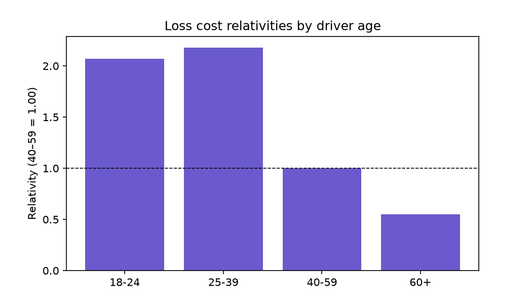
If 18–24 drivers have relativity 2.0, they are expected to cost twice the base band per policy-year. Insurers multiply a base premium by this factor.
Section 5 — Chart relativities
Question
Can the pricing team see the pattern?
Code
plt.figure(figsize=(7, 4))
plt.bar(segment_table["age_band"].astype(str), segment_table["relativity"], color="slateblue")
plt.axhline(1.0, color="black", linewidth=0.8, linestyle="--")
plt.ylabel("Relativity (40–59 = 1.00)")
plt.title("Loss cost relativities by driver age")
plt.savefig("../outputs/charts/module2_relativities.png", dpi=150)
plt.show()
See the sample relativities chart.
What the code does
Visual comparison helps non-technical stakeholders. Always label the base band.
Section 6 — From loss cost to premium (simple)
Question
What premium covers expected losses plus expenses?
Suppose the insurer adds 25% for expenses and profit (combined loading).
Code
loading = 1.25
segment_table["indicative_premium"] = segment_table["loss_cost_per_policy"] * loading
segment_table[["age_band", "loss_cost_per_policy", "indicative_premium"]]
What the code does
Real pricing adds commission, taxes, reinsurance, competitive adjustments and regulatory caps. This is a teaching premium: expected loss × loading.
Section 7 — Fairness note
Create report/module2_fairness_note.md (200–300 words) addressing:
- What the data says about younger vs older drivers.
- One argument for age-based pricing.
- One argument against (or for limiting it).
- Your personal view — should actuaries only supply numbers, or also advise on ethics?
Reflection questions
- Did any relativity surprise you?
- Does writing about fairness feel different from calculating means?
- Could you defend higher premiums to an 18-year-old driver?
Manager feedback
From: Dr. Sarah Okonkwo
Numbers first, values second — but never pretend the values do not exist.
Common trainee mistakes:
- Using average severity across all policies instead of conditioning on claims when explaining "crash size".
- Forgetting exposure — a band with three policies is not evidence.
- Quoting relativities without stating the base band and time period.
If your 18–24 relativity is highest, that matches decades of UK motor experience. If it is not, check your joins — not your politics.
— Sarah
AQA Mathematics links
- Ratio and proportion — relativity factors
- Grouped data — banded averages
- Statistical interpretation — correlation vs causation (age vs experience)
Beyond A-Level
Research generalised linear models (GLMs) for insurance pricing. They extend today's banding to multi-factor models with smooth age curves.
Module 3 — Capital & Reserving
Manager email
From: Dr. Sarah Okonkwo
Subject: IBNR on motor — chain-ladder introNot all claims are reported immediately. At year-end we owe money for accidents that happened but have not been notified yet — Incurred But Not Reported (IBNR).
I have attached cumulative paid claims by accident year and development lag in
paid_triangle.csv. Your tasks:
- Compute age-to-age development factors.
- Project ultimate losses for each accident year.
- Estimate IBNR = ultimate minus latest diagonal paid.
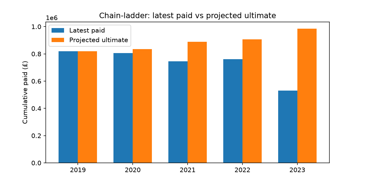
- One chart of observed vs projected ultimate by accident year.
This is a simplified chain-ladder — real reserving adds inflation, large claims and judgement. Learn the mechanics first.
— Sarah
Why this matters
An insurer that under-reserves looks profitable today and collapses tomorrow. Reserving actuaries estimate how much of last year's premium will eventually leave as claims. Regulators and rating agencies watch this closely.
The chain-ladder method is the classic first technique: if past years developed from lag 1 to lag 2 by 1.8× on average, we assume this year's immature year will too.
What you'll learn
- Read a run-off triangle
- Calculate development factors
- Project ultimate claims and IBNR
- See why timing matters in general insurance
Step 1 — Create the paid triangle file
Save the following as data/paid_triangle.csv (copy exactly):
accident_year,lag_1,lag_2,lag_3,lag_4
2019,420000,680000,790000,820000
2020,450000,710000,805000,
2021,480000,745000,,
2022,510000,760000,,
2023,530000,,,
Each row is an accident year (the year policies were in force / accidents occurred). Columns are development lags in months: lag 1 = 12 months after year-end, etc. Values are cumulative paid claims to date (£).
Empty cells are future development not yet observed — that is the triangle shape.
Step 2 — Create the notebook
notebooks/module3_capital_reserving.ipynb
Section 1 — Load the triangle
Question
What does a run-off triangle look like in pandas?
Code
import pandas as pd
import numpy as np
import matplotlib.pyplot as plt

triangle = pd.read_csv("../data/paid_triangle.csv")
triangle
What the code does
Each row is one accident year. Reading left to right, paid claims accumulate as more claims are settled. The bottom-right is empty — 2023 has only one year of development so far.
Section 2 — Extract lag columns
Question
Which columns hold cumulative paid?
Code
lag_cols = ["lag_1", "lag_2", "lag_3", "lag_4"]
paid = triangle.set_index("accident_year")[lag_cols]
paid
What the code does
We keep accident year as the index for readable output.
Section 3 — Age-to-age development factors
Question
How much did each accident year grow between successive lags?
Code
factors = {}
for i in range(len(lag_cols) - 1):
    numer = paid[lag_cols[i + 1]]
    denom = paid[lag_cols[i]]
    factor = (numer / denom).dropna()
    factors[f"{lag_cols[i]}_to_{lag_cols[i+1]}"] = factor

factor_df = pd.DataFrame(factors)
factor_df
What the code does
For 2019→2020 at lag 1→2: divide lag_2 by lag_1 where both exist. Each row gives one observed factor for that development period.
Section 4 — Selected factors (simple average)
Question
What single factor do we use for each development step?
Code
selected = {col: factor_df[col].mean() for col in factor_df.columns}
selected
What the code does
Professional actuaries often use volume-weighted averages or exclude outlier years. A plain mean is fine for this course.
Typical pattern: early development factors are larger (claims still emerging), later ones near 1.0.
Section 5 — Project ultimate losses
Question
Where will each accident year end up?
Code
ultimate = paid.copy()

# Fill 2023: only lag_1 known → multiply through to lag_4
ay = 2023
ultimate.loc[ay, "lag_2"] = ultimate.loc[ay, "lag_1"] * selected["lag_1_to_lag_2"]
ultimate.loc[ay, "lag_3"] = ultimate.loc[ay, "lag_2"] * selected["lag_2_to_lag_3"]
ultimate.loc[ay, "lag_4"] = ultimate.loc[ay, "lag_3"] * selected["lag_3_to_lag_4"]

# 2022: lag_1 and lag_2 known
ay = 2022
ultimate.loc[ay, "lag_3"] = ultimate.loc[ay, "lag_2"] * selected["lag_2_to_lag_3"]
ultimate.loc[ay, "lag_4"] = ultimate.loc[ay, "lag_3"] * selected["lag_3_to_lag_4"]

# 2021
ay = 2021
ultimate.loc[ay, "lag_4"] = ultimate.loc[ay, "lag_3"] * selected["lag_3_to_lag_4"]

ultimate
What the code does
We walk forward along each row, multiplying by selected factors to fill unknown future lags. The ultimate estimate for each year is the projected lag_4 value (fully developed).
2019 is already at lag_4 — no projection needed.
Section 6 — IBNR calculation
Question
How much is still "missing" on the latest diagonal?
Code
latest_paid = paid.apply(lambda row: row.dropna().iloc[-1], axis=1)
projected_ultimate = ultimate["lag_4"]

ibnr_table = pd.DataFrame({
    "latest_paid": latest_paid,
    "projected_ultimate": projected_ultimate,
})
ibnr_table["ibnr"] = ibnr_table["projected_ultimate"] - ibnr_table["latest_paid"]
ibnr_table
What the code does
IBNR for each accident year = projected ultimate − latest observed cumulative paid. Summing IBNR across years gives the reserve the insurer should hold today for past accidents.
Section 7 — Chart observed vs ultimate
Question
Which years are most immature?
Code
years = ibnr_table.index.astype(str)
x = np.arange(len(years))
width = 0.35

plt.figure(figsize=(8, 4))
plt.bar(x - width/2, ibnr_table["latest_paid"], width, label="Latest paid")
plt.bar(x + width/2, ibnr_table["projected_ultimate"], width, label="Projected ultimate")
plt.xticks(x, years)
plt.ylabel("Cumulative paid (£)")
plt.title("Chain-ladder: latest paid vs projected ultimate")
plt.legend()
plt.savefig("../outputs/charts/module3_ibnr.png", dpi=150)
plt.show()
Compare with the sample IBNR chart.
What the code does
2023 should show the largest gap — only one year of development observed. That gap is exactly why insurers hold reserves and capital.
Section 8 — Write Sarah's reserve comment
Add a markdown cell:
- Total IBNR across all years (sum the column).
- Which accident year drives most IBNR?
- Two limitations of chain-ladder (hint: changing claims handling, inflation).
- One sentence on why under-reserving is dangerous for policyholders.
Reflection questions
- Did the triangle format feel like a puzzle or a spreadsheet nightmare?
- Would you trust a method that averages past development without asking why?
- Do you prefer pricing (forward-looking) or reserving (backward-looking)?
Manager feedback
From: Dr. Sarah Okonkwo
Chain-ladder is old, blunt and still everywhere — because it works reasonably when development patterns are stable.
Checklist:
- Immature years dominate IBNR — always say which accident years you are projecting.
- Ultimate ≠ cash tomorrow — it is an estimate of final settlement.
- Reserving is where actuaries fight auditors, regulators and finance — get comfortable defending numbers.
Capital requirements build on reserves plus unexpected shock — Module 4.
— Sarah
AQA Mathematics links
- Ratio and multiplicative change — development factors
- Sequences — cumulative paid across lags
- Estimation — projecting unknown totals from partial data
Beyond A-Level
Look up Bornhuetter–Ferguson reserving. It blends chain-ladder with an external expected loss ratio — useful when data is thin.
Module 4 — Enterprise Risk
Manager email
From: Dr. Sarah Okonkwo
Subject: Flood stress — 1-in-100 scenario for the boardOur client insures homes across England. The board wants to understand enterprise risk from surface-water flooding under a warming climate.
I have put
flood_portfolio.csvin your data folder — 500 policies with region, sum insured and a flood vulnerability score (0–100).Tasks:
- Compute total sum insured by region.
- Apply a stress scenario: every policy with flood score ≥ 70 suffers a 15% partial loss; scores 50–69 suffer 5%; below 50 unaffected.
- Compare stressed losses to a normal-year assumption (2% average loss on sum insured).
- Chart regional stressed losses.
- Short paragraph: what capital buffer might the board want?
— Sarah
Why this matters
Enterprise risk management (ERM) looks across the whole organisation — not one product line in isolation. Climate-related flood is a topical UK stress: more intense rainfall, more surface-water flooding, more concurrent claims across regions.
Actuaries translate physical scenarios into financial impact so directors can decide reinsurance, pricing and capital.
What you'll learn
- Aggregate exposure by region
- Apply a deterministic stress scenario
- Compare normal vs stressed loss assumptions
- Communicate capital implications to non-specialists
Step 1 — Create flood portfolio data
Sarah's email references 500 household policies. Generate the teaching file
once with the code below and save it as data/flood_portfolio.csv:
Code
import pandas as pd
import numpy as np
from pathlib import Path

rng = np.random.default_rng(77)
regions = ["East", "North", "South", "West"]
rows = []

for i in range(1, 501):
    region = regions[(i - 1) % 4]
    sum_insured = int(rng.integers(175, 420) * 1000)
    flood_score = int(np.clip(rng.normal(55, 18), 0, 100))
    rows.append({
        "policy_id": f"H{i:04d}",
        "region": region,
        "sum_insured": sum_insured,
        "flood_score": flood_score,
    })

flood = pd.DataFrame(rows)
flood.to_csv("../data/flood_portfolio.csv", index=False)
flood.head()
Step 2 — Create the notebook
notebooks/module4_enterprise_risk.ipynb
Section 1 — Load portfolio
Question
What exposure are we carrying?
Code
import pandas as pd
import numpy as np
import matplotlib.pyplot as plt

flood = pd.read_csv("../data/flood_portfolio.csv")
flood.head()
Section 2 — Exposure by region
Question
Where is sum insured concentrated?
Code
exposure = (
    flood.groupby("region")["sum_insured"]
    .agg(policies="count", total_sum_insured="sum")
    .assign(avg_sum_insured=lambda d: d["total_sum_insured"] / d["policies"])
)
exposure
What the code does
Sum insured is the maximum the insurer would pay on a total loss. Aggregating by region shows geographic concentration — important for catastrophe risk.
Section 3 — Normal-year loss assumption
Question
What do we expect in an ordinary year?
Code
normal_loss_rate = 0.02
flood["normal_loss"] = flood["sum_insured"] * normal_loss_rate

total_normal = flood["normal_loss"].sum()
total_normal
What the code does
A 2% loss ratio on sum insured is a teaching simplification — real household portfolios use earned premium and peril-specific models.
Section 4 — Apply flood stress scenario
Question
What if a severe rainfall season hits vulnerable properties?
Code
def stress_loss_rate(score):
    if score >= 70:
        return 0.15
    if score >= 50:
        return 0.05
    return 0.0

flood["stress_loss_rate"] = flood["flood_score"].apply(stress_loss_rate)
flood["stress_loss"] = flood["sum_insured"] * flood["stress_loss_rate"]

total_stress = flood["stress_loss"].sum()
uplift = total_stress / total_normal
total_stress, uplift
What the code does
This is a deterministic scenario: not probabilistic, but clear for a board discussion. Scores ≥ 70 might represent properties in known surface-water zones; the 15% partial loss mimics widespread but not total destruction.
Section 5 — Regional stressed losses
Question
Which region suffers most under the scenario?
Code
regional = (
    flood.groupby("region")[["normal_loss", "stress_loss"]]
    .sum()
    .assign(stress_uplift=lambda d: d["stress_loss"] / d["normal_loss"])
)
regional
What the code does
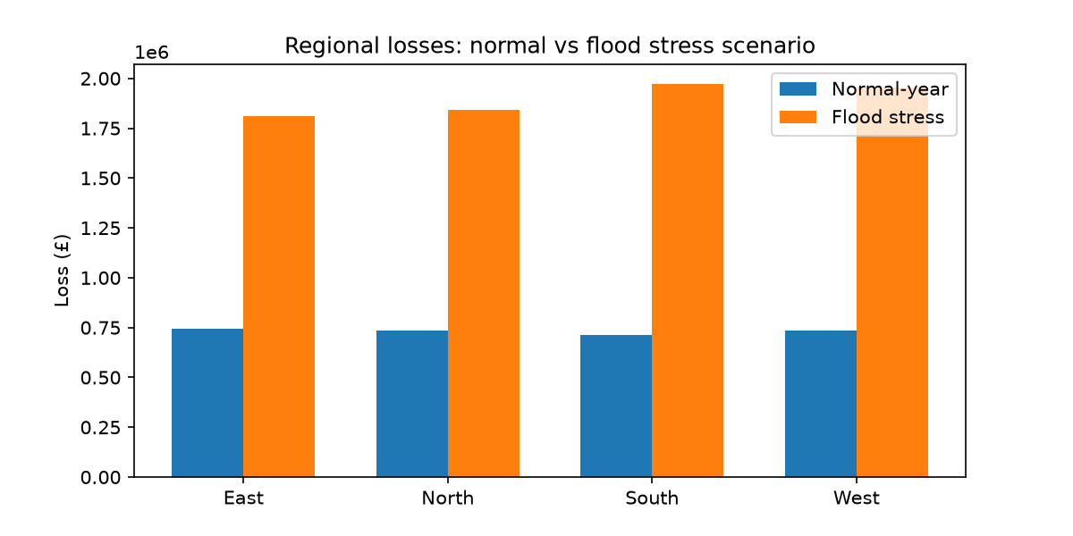
Compare normal vs stress by region. Uplift shows how many times worse the scenario is than the planning assumption.
Section 6 — Chart
Question
Can the board see geographic impact?
Code
regions = regional.index
x = np.arange(len(regions))
width = 0.35

plt.figure(figsize=(8, 4))
plt.bar(x - width/2, regional["normal_loss"], width, label="Normal-year")
plt.bar(x + width/2, regional["stress_loss"], width, label="Flood stress")
plt.xticks(x, regions)
plt.ylabel("Loss (£)")
plt.title("Regional losses: normal vs flood stress scenario")
plt.legend()
plt.savefig("../outputs/charts/module4_flood_stress.png", dpi=150)
plt.show()
See the sample flood stress chart.
Section 7 — Capital buffer discussion
Add a markdown cell (150–250 words):
- Total normal vs stress portfolio loss.
- If the insurer holds capital equal to 1.5× normal-year losses, would that cover the stress scenario?
- Two actions the board could take (reinsurance, reduce high-score exposure, price increase, etc.).
- What information is missing from this toy model?
Reflection questions
- Does climate stress modelling feel like public interest work?
- Would you rather quantify the scenario or choose the scenario assumptions?
- Did this module change how you think about "enterprise" vs single-product risk?
Manager feedback
From: Dr. Sarah Okonkwo
Boards do not need perfect models — they need honest ranges and clear decisions. Your scenario is blunt; real flood modelling uses hazard maps, correlation with windstorm and reinsurance recoveries.
Strong answers mention:
- Concentration — same event, many policies.
- Tail risk — averages miss the year that matters.
- Actions — capital is not the only lever.
Bring this together with motor pricing and IBNR in your final memo.
— Sarah
AQA Mathematics links
- Percentages — partial loss rates on exposure
- Comparison of quantities — stress uplift ratios
- Statistical interpretation — scenario analysis vs forecast
Beyond A-Level
Look up PML (Probable Maximum Loss) and return periods (1-in-100 year events). Regulators often specify which return period insurers must stress.
Module 5 — Professional Project
Manager email
From: Dr. Sarah Okonkwo
Subject: Board memo — motor portfolio reviewOur client’s Risk Committee meets Friday. They want one document tying together your work this month:
- Loss model (frequency × severity)
- Age-based pricing relativities
- IBNR reserve estimate
- Flood stress capital implication
Write a consulting memo (600–800 words) in
report/module5_board_memo.md. Audience: non-actuaries on the board (finance director, CEO, independent directors).Structure:
- Executive summary (3–4 sentences)
- Current motor loss profile
- Pricing adequacy by age band — one recommendation
- Reserve position — headline IBNR number
- Enterprise flood risk — headline stress loss
- Recommended actions (bullet list)
- Limitations — what we have not modelled
Attach or reference charts from Modules 1–4. You may reuse notebook numbers; do not invent statistics you did not calculate.
— Sarah
Why this matters
Trainee actuaries spend as much time writing as modelling. Boards do not read chain-ladder triangles — they read memos that say whether the business is priced safely, reserved honestly and capitalised for bad years.
This is the closest exercise in the course to a real client deliverable.
What you'll learn
- Synthesise technical work for executives
- Balance precision with clarity
- State limitations without undermining your credibility
- Make actionable recommendations under uncertainty
Step 1 — Gather your numbers
Open your notebooks from Modules 1–4 and collect:
| Item | Source notebook | Typical symbol |
|---|---|---|
| Poisson λ | module1 | lambda_hat |
| Pure premium per policy | module1 | pure_premium |
| Highest age-band relativity | module2 | segment_table |
| Total IBNR | module3 | ibnr_table["ibnr"].sum() |
| Flood stress total loss | module4 | total_stress |
Create notebooks/module5_board_project.ipynb and run a recap cell:
Code
import pandas as pd
import numpy as np

# --- Module 1 recap ---
policies = pd.read_csv("../data/motor_policies.csv")
claims = pd.read_csv("../data/motor_claims.csv")
lambda_hat = policies["claim_count"].mean()
mean_severity = claims["claim_amount"].mean()
pure_premium = lambda_hat * mean_severity

# --- Module 2 recap ---
cost_by_policy = claims.groupby("policy_id")["claim_amount"].sum()
policy_data = policies.merge(
    cost_by_policy.rename("total_claim_cost"),
    on="policy_id",
    how="left",
)
policy_data["total_claim_cost"] = policy_data["total_claim_cost"].fillna(0)
bins = [17, 24, 39, 59, 100]
labels = ["18-24", "25-39", "40-59", "60+"]
policy_data["age_band"] = pd.cut(policy_data["driver_age"], bins=bins, labels=labels)
seg = policy_data.groupby("age_band", observed=True)["total_claim_cost"].mean()
base = seg["40-59"]
relativities = (seg / base).round(2)

# --- Module 3 recap ---
triangle = pd.read_csv("../data/paid_triangle.csv")
lag_cols = ["lag_1", "lag_2", "lag_3", "lag_4"]
paid = triangle.set_index("accident_year")[lag_cols]
factor_df = pd.DataFrame({
    f"{lag_cols[i]}_to_{lag_cols[i+1]}": (
        paid[lag_cols[i + 1]] / paid[lag_cols[i]]
    ).dropna()
    for i in range(len(lag_cols) - 1)
})
selected = {c: factor_df[c].mean() for c in factor_df.columns}
ultimate = paid.copy()
for ay in [2023, 2022, 2021]:
    if pd.isna(ultimate.loc[ay, "lag_2"]):
        ultimate.loc[ay, "lag_2"] = ultimate.loc[ay, "lag_1"] * selected["lag_1_to_lag_2"]
    if pd.isna(ultimate.loc[ay, "lag_3"]):
        ultimate.loc[ay, "lag_3"] = ultimate.loc[ay, "lag_2"] * selected["lag_2_to_lag_3"]
    if pd.isna(ultimate.loc[ay, "lag_4"]):
        ultimate.loc[ay, "lag_4"] = ultimate.loc[ay, "lag_3"] * selected["lag_3_to_lag_4"]
latest_paid = paid.apply(lambda row: row.dropna().iloc[-1], axis=1)
ibnr = (ultimate["lag_4"] - latest_paid).sum()

# --- Module 4 recap ---
flood = pd.read_csv("../data/flood_portfolio.csv")
def stress_loss_rate(score):
    if score >= 70: return 0.15
    if score >= 50: return 0.05
    return 0.0
flood["stress_loss"] = flood["sum_insured"] * flood["flood_score"].map(
    lambda s: stress_loss_rate(s)
)
total_stress = flood["stress_loss"].sum()
normal_total = flood["sum_insured"].sum() * 0.02

pd.Series({
    "lambda_hat": lambda_hat,
    "pure_premium": pure_premium,
    "max_relativity_band": relativities.idxmax(),
    "max_relativity": relativities.max(),
    "total_ibnr": ibnr,
    "flood_stress_loss": total_stress,
    "flood_normal_loss": normal_total,
})
What the code does
One place to copy numbers into your memo — reduces transcription errors.
Section 2 — Memo template
Create report/module5_board_memo.md. Below is a structure only — replace
bracketed text with your calculated values and your own prose.
# Consulting memo — Motor & household portfolio review
**To:** Risk Committee, [Client Insurer plc]
**From:** Dr. Sarah Okonkwo, Horizon Risk Consulting
**Date:** [today]
**Prepared by:** [Your name], Actuarial Analyst
## Executive summary
[3–4 sentences: overall portfolio health, biggest risk, top recommendation.]
## 1. Motor loss model
Our compound model estimates an average claim frequency of [λ] claims per
policy-year and a mean severity of £[X] per claim. Expected loss cost (pure
premium) is approximately £[P] per policy-year. Simulation shows material
spread around this mean — a single year can deviate significantly.

## 2. Pricing by driver age
Age band analysis (base: 40–59) shows the highest relativity in the [band]
segment at [R]× the base loss cost. Indicative premiums with 25% loading
range from £[low] to £[high] across bands.
**Recommendation:** [One concrete pricing action — e.g. review 18–24
relativity, cap increases, monitoring exposure.]

## 3. Reserves (IBNR)
Chain-ladder projection on paid claims triangles yields total IBNR of
£[IBNR] across accident years 2019–2023. The 2023 accident year contributes
the largest share because it is most immature.

## 4. Enterprise flood stress
Under the agreed 1-in-100 style surface-water scenario, portfolio stress losses
total £[S] compared with a normal-year planning assumption of £[N] ([uplift]×
uplift). Regional concentrations in [region] warrant attention.

## 5. Recommended actions
- [Action 1 — e.g. hold additional capital for flood tail.]
- [Action 2 — e.g. review young-driver pricing.]
- [Action 3 — e.g. reinsurance or aggregate limits.]
## 6. Limitations
- Synthetic / simplified data and methods throughout.
- Chain-ladder ignores inflation and claims process changes.
- Flood scenario is deterministic, not probabilistic.
- No correlation between motor and household lines modelled.
- [Your own limitation from the work you found hardest.]
---
*This memo is for training purposes and does not constitute professional advice.*Section 3 — Quality checklist
Before submitting to Sarah (your teacher or future you), verify:
- Every number in the memo appears in a notebook output.
- Recommendations follow from numbers — not generic insurance clichés.
- Limitations are honest — boards trust analysts who know what they do not know.
- Charts render when you open the markdown preview (paths relative to
report/). - Word count 600–800 in sections 1–6 (excluding headers).
A sample memo is on Worked examples.
Section 4 — Optional oral defence
Prepare three minutes of spoken answers (record yourself or practice aloud):
- If the CEO asks "Are we overcharging young drivers?" — what do you say?
- If the finance director asks "Why should I trust IBNR?" — what do you say?
- If a director asks "Should we exit flood-prone postcodes?" — what do you say?
Actuaries are hired for judgement under questioning, not memos in a drawer.
Reflection questions
- Which module felt most like real actuarial work?
- Did you prefer Python, writing, or the business discussion?
- After five modules in 201 (and five in 101), do you want to pursue actuarial exams — or was one week enough to decide?
- What would you need to learn next to do this job for real?
Manager feedback
From: Dr. Sarah Okonkwo
If I put this memo in front of a board, I would look for:
- Headline numbers in the executive summary — busy people stop reading without them.
- Recommendations that cost something — vague "monitor risk" lines waste meetings.
- Limitations that match the methods — copy-paste disclaimers fool no one.
You are not an actuary yet. But you now think in frequency, severity, reserve, capital and communication. That is the profession in miniature.
If you want to go further, the IFoA publishes the Curriculum 2025 syllabus — look at CS1 (risk modelling) and CP1 (actuarial practice) to see what university + exams add on top of this taster.
Thank you for your work this month. — Sarah
AQA Mathematics links
- Problem synthesis — combining statistical, financial and written reasoning
- Modelling cycle — assumptions, computation, validation, communication
- Critical thinking — limitations and recommendations
Beyond A-Level
Explore the IFoA student membership path and apprenticeship actuary roles. Many UK actuaries train while working — exams are hard but not the only route story worth hearing.
Module 6 — What You Have Learned
By the end of Actuarial Science 201, you have learned to:
- build a compound loss model with Poisson frequency and empirical severity;
- segment motor pricing by driver age and debate fairness;
- estimate IBNR with a chain-ladder run-off triangle;
- stress-test flood exposure for enterprise risk;
- deliver a board consulting memo synthesising the work.
If you enjoyed measuring uncertainty, pricing risk, reserving honestly and writing for decision-makers, actuarial science may be worth exploring further.
Return to Actuarial Science 101 if you have not completed the introductory week yet — 201 assumes that foundation.
Continue to Actuarial Science 301 for an open-ended project of your own design.