Actuarial Science · Level 101
Actuarial Science 101 — Could I Be an Actuary?
Shadow a junior actuary — from claims data to premiums, pensions and a Risk Committee recommendation.
Actuarial Science · Level 101
Actuarial Science 101 — Could I Be an Actuary?
Shadow a junior actuary — from claims data to premiums, pensions and a Risk Committee recommendation.
Actuarial Science 101 — Could I Be an Actuary?
Prerequisite: Data Science 101.
This course assumes you can already use VS Code, Jupyter Notebooks, Python, pandas and matplotlib. We won't reteach those. Instead, you'll discover how actuaries use those tools to measure uncertainty and support decisions about insurance, pensions and long-term risk.
You have joined Horizon Risk Consulting, a London firm that advises insurers, pension schemes and public bodies on risk. Your manager is Dr. Sarah Okonkwo, Chief Actuary.
Over five modules you will do real junior-actuary work:
- Understand what actuaries do and whether the career appeals to you.
- Measure insurance risk using claims data — frequency and severity.
- Build a simple car insurance premium and discuss fairness.
- Use a mortality table to estimate pension costs when people live longer.
- Deliver a short brief to the Risk Committee on premiums, pensions or flood risk.
Sample student outputs: Worked examples. Your charts should look broadly similar (claims summary, premiums, survival stress) — not identical.
The mindset to keep throughout:
event → probability → cost → decision
Before you start — create your project folder
Open File Explorer (or Finder on Mac).
Create a folder called actuarial101 inside your existing coding folder
(the same parent folder you used for Data Science).
Inside actuarial101, create:
Open VS Code. Choose File → Open Folder and open actuarial101.
You will save CSV files in data/, notebooks in notebooks/, charts in
outputs/charts/, and short written answers in report/.
Tools
- VS Code
- Jupyter Notebook
- Python
- pandas
- matplotlib
If you need a package you have not installed yet:
pip install pandas matplotlib jupyter ipykernelModule 1 — What is an Actuary?
Manager email
From: Dr. Sarah Okonkwo
Subject: Welcome to Horizon Risk ConsultingWelcome aboard. Before I give you any claims data, I need to know whether you understand what an actuary actually does — and whether you find that kind of work interesting.
This week, read about three UK employers: Aviva, Mercer and the Government Actuary's Department (GAD). All employ actuaries. Check each organisation's careers page and its early-careers or internships section — those pages often explain what the work is really like. Then send me a one-page note answering:
- What does an actuary do day to day?
- Why do organisations pay actuaries to think about the future?
- Which employer sounds most interesting to you, and why?
No Python required today. Think like an analyst, not a programmer.
— Sarah
Why this matters
Boards and regulators do not hire actuaries because they enjoy spreadsheets. They hire actuaries because the future is uncertain and expensive mistakes are possible.
An actuary's job is to:
- turn messy real-world events into measurable probabilities;
- estimate what those events might cost;
- explain results clearly to people who must decide today.
If you dislike careful reasoning under uncertainty, you will not enjoy this career — even if you are good at Python.
What you'll learn
- What an actuary does in insurance, pensions and consulting
- The difference between life insurers, pension consultants and government actuaries
- What a pension scheme is and why longevity matters
- Typical UK career paths, professional exams and graduate salaries
- Whether this style of work feels motivating to you
What is insurance?
When you buy car insurance, you pay a small amount regularly. If you have an accident, the insurer pays a much larger repair bill.
The insurer does not know whether you will crash this year. But they can study thousands of drivers and estimate how often crashes happen and how much they cost. That is the actuarial starting point:
How often? (frequency) How much? (severity)
Three types of employer
| Type | Example | Actuarial work often involves… |
|---|---|---|
| Life & general insurer | Aviva | Pricing policies, reserving for claims, capital |
| Pension & benefits consultant | Mercer | Pension funding, longevity, employer schemes |
| Government actuary | GAD | National insurance, state pensions, public finance |
Horizon Risk Consulting is closest to a consulting firm: we advise clients who cannot afford to guess about long-term obligations.
What is a pension?
A defined benefit pension promises retired workers a monthly income for life. If people live longer than expected, the scheme must pay out for more years — sometimes decades after the employer thought the obligation was "finished."
Actuaries estimate how long members might live and whether today's contributions are enough. That is not prediction for its own sake. It supports decisions about contributions, benefits and company balance sheets.
Your tasks
Create a new file:
report/module1_actuary_research.md
Answer the following in clear prose (roughly 300–500 words total).
Task 1 — Research three employers
Visit the careers pages of Aviva, Mercer and the Government Actuary's Department. For each organisation, also check its early-careers or internships section if one exists — many actuarial employers hire through graduate programmes and year-in-industry placements rather than ad-hoc roles. For example, Aviva publishes its early-careers pathways at careers.aviva.co.uk/early-careers/.
For each employer, note:
- what the organisation says it does;
- one example role that mentions actuarial work, mathematics or risk;
- where in the UK it hires;
- whether it offers internships or graduate programmes (and what they involve, if so).
Task 2 — Compare graduate pay (roughly)
Search "actuarial graduate salary UK" and read two recent sources (job boards, BrightNetwork, firm pages). You do not need exact figures — estimate a range and cite your sources.
Task 3 — Explain the premium
In your own words: why might a firm pay an actuarial graduate more than many other graduate roles? Connect your answer to long-term obligations, regulation and money at risk if estimates are wrong.
Task 4 — Pick one employer
Which of the three would you most like to learn more about? One honest paragraph — there is no correct answer.
Reflection questions
Add a short section at the bottom of your report:
- Did you enjoy the research, or did you find it tedious?
- Did the salary information change your interest, or not really?
- Did any job description sound exciting? Any sound miserable?
- Do you like the idea of being responsible when a model affects real people's pensions or insurance premiums?
Manager feedback
From: Dr. Sarah Okonkwo
Good first effort. A few things strong actuaries always do in week one:
- They distinguish facts from marketing language on careers pages.
- They check internship and early-careers pages as well as graduate listings — that is often where you learn what day-to-day work actually looks like.
- They notice whether they enjoy thinking about the long term — that matters more than liking maths in abstract.
- They ask who suffers when an estimate is wrong: policyholders, pensioners, taxpayers or shareholders.
If you felt curious and wanted to dig deeper, that is a good sign. If you were bored unless something flashed on a screen, notice that too.
Tomorrow we look at real claims data. Bring your Python environment.
— Sarah
AQA Mathematics links
- Statistics — interpreting data and sources critically
- Probability — uncertainty as a core idea in insurance and pensions
Beyond A-Level
Look up the Institute and Faculty of Actuaries (IFoA). UK actuaries qualify through professional exams taken while working — a different path from a three-year maths degree alone.
Module 2 — Measuring Risk
Manager email
From: Dr. Sarah Okonkwo
Subject: Motor claims — how bad is our book?A regional insurer has sent us three years of motor insurance claims. Before we advise on pricing, I need the basics measured cleanly:
- How often do policyholders claim? (frequency)
- When they claim, how much does it cost? (severity)
- What is the expected cost per policy?
Generate a synthetic dataset (I'll explain why consultants sometimes simulate data), save it as
motor_claims.csv, and summarise the book in one chart I can paste into a client slide deck.— Sarah
Why this matters
Before Horizon recommends a premium, someone on my team answers boring-sounding questions:
- What fraction of drivers claim each year?
- Are a few huge claims driving the average?
- What should we expect to pay per policy on average?
That is not "prediction" yet. It is measurement — the step actuaries never skip.
What you'll learn
- Generate and save synthetic claims data with pandas
- Split insurance risk into frequency and severity
- Calculate expected value as a probability-weighted average cost
- Visualise the distribution of claim sizes
Step 1 — Create the notebook
In VS Code, create:
notebooks/module2_measuring_risk.ipynb
Select your Python kernel (same as Data Science).
Section 1 — Generate synthetic motor claims
Question
Can we create a realistic-looking claims dataset in Python?
Real insurers guard their data carefully. Consultants often start with synthetic or anonymised data to build models before seeing client files. We will simulate 5,000 policy-years of motor cover.
Code
import numpy as np
import pandas as pd

np.random.seed(42)

n_policies = 5000
claim_probability = 0.08  # 8% of policy-years have at least one claim

has_claim = np.random.random(n_policies) < claim_probability

# Severity in pounds: many small bumps, occasional large repairs
severity = np.where(
    has_claim,
    np.random.lognormal(mean=7.5, sigma=0.9, size=n_policies),
    0.0,
)

claims = pd.DataFrame({
    "policy_id": [f"POL-{i:05d}" for i in range(1, n_policies + 1)],
    "year": np.random.choice([2022, 2023, 2024], size=n_policies),
    "driver_age": np.random.randint(18, 75, size=n_policies),
    "has_claim": has_claim.astype(int),
    "claim_amount": severity.round(2),
})

claims.head(10)
What the code does
We simulate 5,000 policy-years. Each row is one car insured for one year.
claim_probability = 0.08 means about 8% of rows have a claim — our
frequency assumption.
When there is a claim, lognormal draws a repair cost skewed toward smaller
amounts with occasional large ones — realistic severity shape.
Rows with no claim have claim_amount = 0.
Section 2 — Save the dataset
Question
Can we reuse this file like a real client CSV?
Code
claims.to_csv("../data/motor_claims.csv", index=False)
print("Saved", len(claims), "rows to ../data/motor_claims.csv")
What the code does
to_csv writes the DataFrame to your data/ folder. From now on, load
this file as if it arrived from the insurer — do not regenerate unless you
want a fresh random sample.
Section 3 — Load and inspect
Question
Does the saved file look sensible?
Code
claims = pd.read_csv("../data/motor_claims.csv")
claims.info()
claims.describe()
What the code does
read_csv loads the file. info() shows column types and row count.
describe() summarises numeric columns — check claim_amount max versus
median.
Section 4 — Frequency
Question
How often do policyholders claim?
Code
frequency = claims["has_claim"].mean()
n_claims = claims["has_claim"].sum()

frequency, n_claims
What the code does
mean() on a 0/1 column equals the proportion of ones — here, the
claim frequency (probability of at least one claim in a policy-year).
Section 5 — Severity (conditional on a claim)
Question
When someone claims, how much does it cost on average?
Code
paid_claims = claims.loc[claims["has_claim"] == 1, "claim_amount"]

avg_severity = paid_claims.mean()
median_severity = paid_claims.median()
max_severity = paid_claims.max()

avg_severity, median_severity, max_severity
What the code does
We filter to rows with a claim only. The average severity is the mean repair cost among claimants.
Compare mean and median. If mean >> median, a few large claims are pulling the average up — common in insurance.
Section 6 — Expected cost per policy
Question
What should the insurer expect to pay per policy-year?
Code
expected_cost_per_policy = (claims["has_claim"] * claims["claim_amount"]).mean()

# Equivalent decomposition: frequency × average severity
frequency * avg_severity, expected_cost_per_policy
What the code does
For each policy, has_claim * claim_amount equals the paid amount (zero if
no claim). The mean is the expected cost per policy.
For this simple setup (at most one claim per year):
That decomposition is how actuaries often build premium models.
Section 7 — Chart claim amounts
Question
Can Sarah see the shape of severity?
Code
import matplotlib.pyplot as plt

fig, axes = plt.subplots(1, 2, figsize=(10, 4))

axes[0].hist(paid_claims, bins=40, edgecolor="white")
axes[0].set_title("Claim amounts (when claim > 0)")
axes[0].set_xlabel("Amount (£)")
axes[0].set_ylabel("Count")

age_bins = pd.cut(claims["driver_age"], bins=[17, 25, 40, 60, 75])
freq_by_age = claims.groupby(age_bins, observed=True)["has_claim"].mean()
freq_by_age.plot(kind="bar", ax=axes[1], rot=45)
axes[1].set_title("Claim frequency by driver age band")
axes[1].set_ylabel("Frequency")

plt.tight_layout()
plt.savefig("../outputs/charts/module2_claims_summary.png", dpi=150)
plt.show()
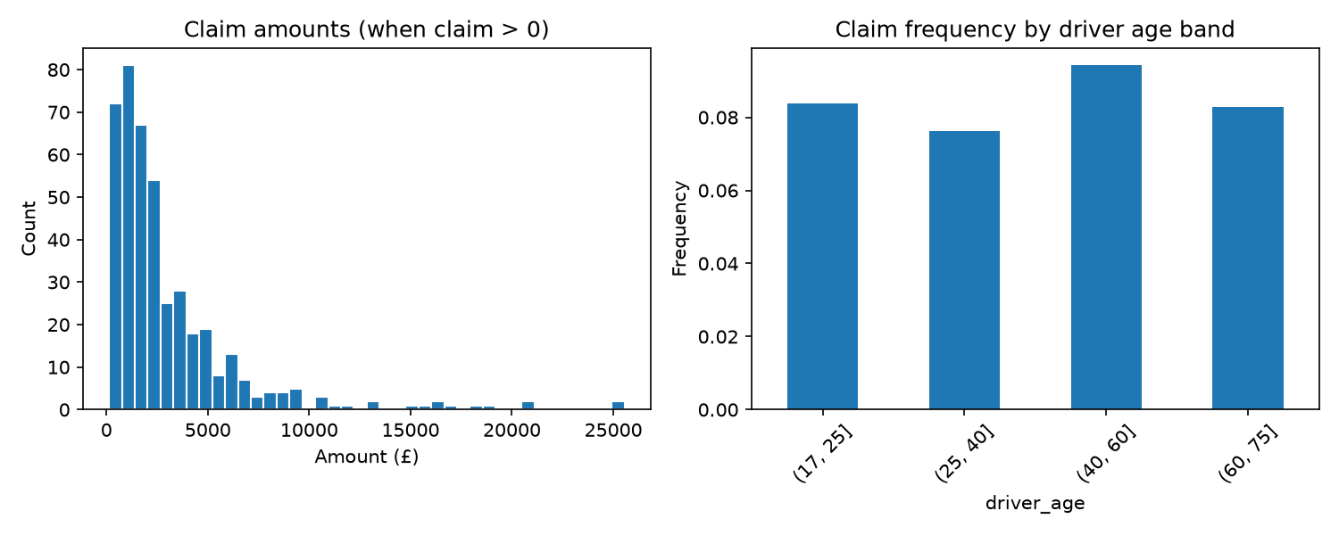
Compare with the sample claims summary.
What the code does
The left histogram shows severity — mostly moderate repairs, a long right tail.
The right chart groups frequency by age band. Younger drivers often claim more often — insurers notice patterns like this when pricing.
Section 8 — Write Sarah's summary
Add a markdown cell answering:
- What is the claim frequency in your sample?
- What is average severity among claimants?
- What is expected cost per policy?
- Is mean severity much larger than median? What does that imply?
- Which age band has the highest frequency?
Reflection questions
- Did you enjoy separating frequency from severity?
- Did any result surprise you?
- Would you trust one average without plotting the distribution?
Manager feedback
From: Dr. Sarah Okonkwo
Solid work. Two habits to keep:
- Always decompose — total cost = how often × how much.
- Always plot — averages hide a few catastrophic claims.
Next you will turn expected cost into a premium a customer might pay. That step brings ethics into the room.
— Sarah
AQA Mathematics links
- Expected value — probability-weighted average outcome
- Averages and spread — mean versus median for skewed data
Beyond A-Level
Look up compound Poisson models. Insurers often model claim counts and severate separately, then combine them — exactly the structure you used today.
Module 3 — Putting a Price on Risk
Manager email
From: Dr. Sarah Okonkwo
Subject: A simple motor premium — and a fairness questionThe insurer wants a transparent premium calculator for three driver profiles:
- Profile A: age 22, one at-fault accident last year
- Profile B: age 35, clean record
- Profile C: age 55, clean record
Start from expected claims cost, add a loading for expenses and profit, and quote an annual premium for each.
Then write me half a page on fairness: is it ethical to charge young drivers more? What would you tell a customer who asks?
— Sarah
Why this matters
A premium is not "whatever the market will bear." It starts from expected cost, then adds margin for:
- administration and claims handling;
- reinsurance and capital;
- profit (or surplus for mutual insurers).
Actuaries also face fairness questions: statistical groups differ, but regulators and society ask whether pricing rules are acceptable.
What you'll learn
- Build a simple premium from expected cost plus loading
- Apply age and claims-history factors from data
- Discuss trade-offs between actuarial fairness and social fairness
- Communicate pricing in plain English
Step 1 — Create the notebook
notebooks/module3_pricing.ipynb
Section 1 — Load claims data
Question
Do we still have the motor claims file?
Code
import pandas as pd
import numpy as np

claims = pd.read_csv("../data/motor_claims.csv")
claims.head()
What the code does
Same CSV from Module 2 — real projects reuse data across tasks.
Section 2 — Age factors from the data
Question
How much riskier are younger drivers in our sample?
Code
age_bins = pd.cut(claims["driver_age"], bins=[17, 25, 40, 60, 75],
                  labels=["18-25", "26-40", "41-60", "61-75"])

base_freq = claims["has_claim"].mean()
freq_table = claims.groupby(age_bins, observed=True)["has_claim"].mean()
rel_freq = (freq_table / base_freq).round(3)

freq_table, rel_freq
What the code does
We compute claim frequency by age band, then divide by the base frequency to get relative factors. A factor of 1.5 means 50% more claims than average.
These are illustrative — real insurers use much richer data and regulation.
Section 3 — Base expected cost
Question
What is the portfolio-average expected cost?
Code
frequency = claims["has_claim"].mean()
avg_severity = claims.loc[claims["has_claim"] == 1, "claim_amount"].mean()
base_expected_cost = frequency * avg_severity

base_expected_cost
What the code does
Same decomposition as Module 2. This is the starting pure premium before expenses and profit.
Section 4 — Premium formula
Question
How do we turn expected cost into a customer premium?
A simple formula:
We will use loading = 25% for expenses and profit combined.
Code
LOADING = 0.25

def quote_premium(age, at_fault_last_year=False):
    if age <= 25:
        age_factor = rel_freq["18-25"]
    elif age <= 40:
        age_factor = rel_freq["26-40"]
    elif age <= 60:
        age_factor = rel_freq["41-60"]
    else:
        age_factor = rel_freq["61-75"]

    history_factor = 1.35 if at_fault_last_year else 1.0

    expected = base_expected_cost * age_factor * history_factor
    premium = expected * (1 + LOADING)
    return round(premium, 2)

quote_premium(22, at_fault_last_year=True)
What the code does
quote_premium maps a driver profile to factors, multiplies the base
expected cost, then adds 25% loading.
history_factor = 1.35 is a simplified penalty for a recent at-fault
accident — real insurers use formal bonus-malus systems.
Section 5 — Quote three profiles
Question
What premiums do Sarah's three profiles receive?
Code
profiles = pd.DataFrame([
    {"profile": "A", "age": 22, "at_fault_last_year": True},
    {"profile": "B", "age": 35, "at_fault_last_year": False},
    {"profile": "C", "age": 55, "at_fault_last_year": False},
])

profiles["annual_premium"] = profiles.apply(
    lambda row: quote_premium(row["age"], row["at_fault_last_year"]),
    axis=1,
)

profiles
What the code does
We apply the calculator to each profile and collect quoted premiums in a table — the kind of output a pricing analyst sends to a manager.
Section 6 — Visualise premiums
Question
Can Sarah see how profiles compare?
Code
import matplotlib.pyplot as plt

plt.figure(figsize=(6, 4))
plt.bar(profiles["profile"], profiles["annual_premium"])
plt.ylabel("Annual premium (£)")
plt.title("Quoted motor premiums (simplified model)")
for i, v in enumerate(profiles["annual_premium"]):
    plt.text(i, v + 20, f"£{v:,.0f}", ha="center")
plt.savefig("../outputs/charts/module3_premium_quotes.png", dpi=150)
plt.show()
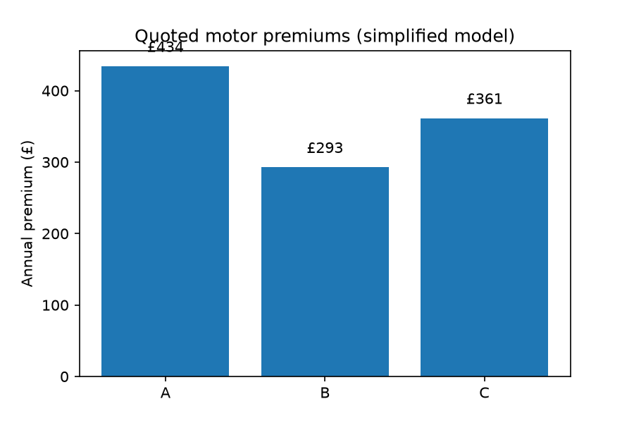
See the sample premium quotes chart.
What the code does
A simple bar chart makes the spread between young/high-risk and older/clean drivers visible — useful when discussing fairness with non-actuaries.
Section 7 — Fairness discussion
Create report/module3_fairness.md (200–300 words) answering:
- Why is Profile A charged more than Profile C? Use frequency and expected cost in your explanation.
- Is it actuarially fair to charge different prices for different risk groups?
- Is it always socially fair? What might a 22-year-old driver argue?
- What would you tell a customer who says: "I have never crashed — why should I pay for other people's accidents?"
There is no single correct answer. Horizon wants to see you hold both the numbers and the human side.
Reflection questions
- Did you feel uncomfortable quoting a high premium for Profile A?
- Do you enjoy the policy discussion as much as the coding?
- Would you rather build the formula or explain it to a client?
Manager feedback
From: Dr. Sarah Okonkwo
Good. Actuaries who only optimise formulas forget that premiums are prices real people pay. Actuaries who only talk ethics forget that insurers must remain solvent.
The job is to connect both: measure risk honestly, then explain the decision transparently.
Next we look further into the future — pensions and mortality.
— Sarah
AQA Mathematics links
- Ratio and proportion — relative risk factors
- Expected value — pure premium as weighted average cost
Beyond A-Level
Research EU gender directive and UK Equality Act implications for insurance pricing. Not all statistically relevant factors may be used in premiums.
Module 4 — Planning for an Uncertain Future
Manager email
From: Dr. Sarah Okonkwo
Subject: Pension scheme review — what if we all live longer?A corporate client sponsors a defined benefit pension for 1,000 retired members. Each receives £12,000 per year for life.
Use the simplified mortality table below (not real GAD tables — those are huge). Estimate:
- Expected total pension payments over members' lifetimes at current mortality.
- How total cost changes if life expectancy rises by three years (shift deaths later).
Write one paragraph on why the finance director should care today.
— Sarah
Why this matters
Pension promises can last forty years. A small change in longevity assumptions can move liabilities by millions of pounds. Actuaries do not wait for everyone to die before updating estimates — schemes fund and reserve based on today's best view of the future.
What you'll learn
- Read a basic mortality table (qx = probability of death in year x)
- Estimate expected pension payments from survival probabilities
- Stress-test assumptions when life expectancy improves
- Connect longevity risk to employer balance sheets
The mortality table
We use a simplified table for ages 65–90. qx is the probability a person
alive at the start of age x dies during that year.
| Age | qx |
|---|---|
| 65 | 0.010 |
| 66 | 0.011 |
| 67 | 0.012 |
| 68 | 0.013 |
| 69 | 0.014 |
| 70 | 0.016 |
| 71 | 0.018 |
| 72 | 0.020 |
| 73 | 0.022 |
| 74 | 0.025 |
| 75 | 0.028 |
| 76 | 0.032 |
| 77 | 0.036 |
| 78 | 0.041 |
| 79 | 0.047 |
| 80 | 0.054 |
| 81 | 0.062 |
| 82 | 0.071 |
| 83 | 0.081 |
| 84 | 0.093 |
| 85 | 0.107 |
| 86 | 0.123 |
| 87 | 0.141 |
| 88 | 0.162 |
| 89 | 0.186 |
| 90 | 1.000 |
Assume all 1,000 members are age 65 now and receive £12,000 at the start of each year they survive.
Step 1 — Create the notebook
notebooks/module4_pensions.ipynb
Section 1 — Build the mortality table in pandas
Question
Can we load the embedded table cleanly?
Code
import pandas as pd
import numpy as np
import matplotlib.pyplot as plt

mortality = pd.DataFrame({
    "age": range(65, 91),
    "qx": [
        0.010, 0.011, 0.012, 0.013, 0.014, 0.016, 0.018, 0.020,
        0.022, 0.025, 0.028, 0.032, 0.036, 0.041, 0.047, 0.054,
        0.062, 0.071, 0.081, 0.093, 0.107, 0.123, 0.141, 0.162,
        0.186, 1.000,
    ],
})

mortality.head()
What the code does
We embed the table directly — real projects use published tables (ONS, CMI) with hundreds of rows and separate rates for men and women.
Section 2 — Survival probabilities
Question
What fraction of members are alive at each age?
Code
mortality["px"] = 1 - mortality["qx"]
mortality["survival_to_start_of_age"] = mortality["px"].cumprod().shift(
    fill_value=1.0
)

mortality[["age", "qx", "survival_to_start_of_age"]].head(8)
What the code does
px is one-year survival probability. The cumulative product of px values
gives the probability of surviving from age 65 to the start of age 66,
67, and so on.
The first row uses fill_value=1.0 — everyone is alive at 65.
Section 3 — Expected payments per member
Question
How much do we expect to pay one typical member?
Code
ANNUAL_PENSION = 12_000

mortality["expected_payment"] = (
    mortality["survival_to_start_of_age"] * ANNUAL_PENSION
)

expected_per_member = mortality["expected_payment"].sum()
expected_per_member
What the code does
If survival probability to age 70 is 0.92, we expect to pay £12,000 × 0.92 that year. Summing across ages gives expected lifetime pension cost per member — the actuarial present value of benefits (ignoring discounting for simplicity).
Section 4 — Total scheme cost
Question
What does the employer face for 1,000 retirees?
Code
MEMBERS = 1000
total_expected = expected_per_member * MEMBERS
total_expected
What the code does
Multiply per-member expectation by headcount. This is the kind of number a finance director sees when longevity assumptions move.
Section 5 — Stress test: +3 years life expectancy
Question
What if medical progress delays deaths?
A simple stress: shift qx values three years later — deaths that would have happened at 70 happen at 73 instead. We approximate this by moving the death probabilities down the table.
Code
shift = 3
stressed = mortality.copy()
stressed["qx_stressed"] = stressed["qx"].shift(shift, fill_value=0.0)
stressed.loc[stressed.index[-shift:], "qx_stressed"] = stressed.loc[
    stressed.index[-shift:], "qx"
]

stressed["px_stressed"] = 1 - stressed["qx_stressed"]
stressed["survival_stressed"] = stressed["px_stressed"].cumprod().shift(
    fill_value=1.0
)
stressed["payment_stressed"] = stressed["survival_stressed"] * ANNUAL_PENSION

stressed_per_member = stressed["payment_stressed"].sum()
stressed_total = stressed_per_member * MEMBERS

increase = stressed_total - total_expected
increase, increase / total_expected
What the code does
shift(3) pushes mortality rates to older ages — members survive longer on
average. We recompute expected payments and compare totals.
The percentage increase shows why pension actuaries treat longevity as a major risk factor.
Section 6 — Chart survival curves
Question
Can Sarah see the stress test visually?
Code
plt.figure(figsize=(8, 4))
plt.plot(mortality["age"], mortality["survival_to_start_of_age"],
         label="Base mortality")
plt.plot(stressed["age"], stressed["survival_stressed"],
         label="Stressed (+3 years)")
plt.xlabel("Age")
plt.ylabel("Probability alive at start of age")
plt.title("Survival curve: base vs stressed longevity")
plt.legend()
plt.savefig("../outputs/charts/module4_survival_stress.png", dpi=150)
plt.show()
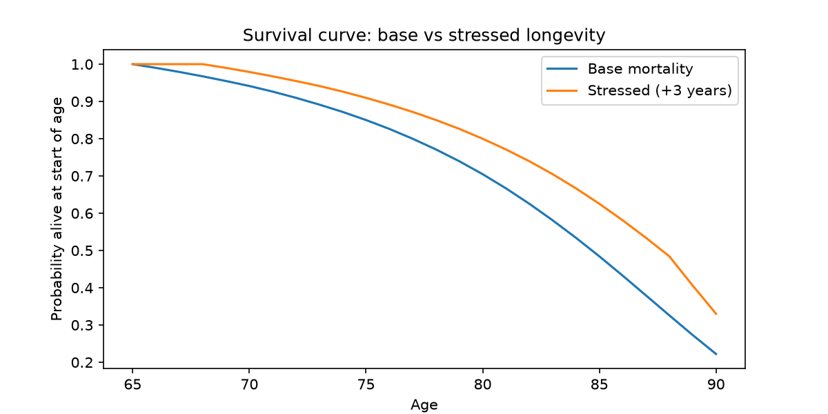
Compare with the sample survival stress chart.
What the code does
The stressed curve sits above the base curve — more people alive at each age, so more pension payments.
Section 7 — Write the finance director note
Create report/module4_pension_note.md (150–250 words) answering:
- What is expected total pension cost under base mortality?
- How much does cost increase under the +3 year stress?
- Why should the finance director care now, even though payments stretch decades ahead?
- One limitation of this simplified model (hint: discounting, inflation, new retirees joining).
Reflection questions
- Did thinking in decades feel natural or strange?
- Do you prefer insurance pricing (Module 3) or pension projections?
- Would you enjoy explaining these numbers to a non-technical board?
Manager feedback
From: Dr. Sarah Okonkwo
Strong analysts connect longevity to cash the employer must set aside today. A 5% liability increase can mean higher contributions next quarter — not "someone else's problem in 2050."
If you ignored limitations like discount rates, good — noticing what a model skips is actuarial thinking.
— Sarah
AQA Mathematics links
- Probability — survival and mortality as complementary events
- Sequences — cumulative products of year-on-year survival
Beyond A-Level
Look up discounting and present value. Actuaries convert future pension payments to a single liability figure using interest rates — essential for balance sheet reporting.
Module 5 — Final Project
Manager email
From: Dr. Sarah Okonkwo
Subject: Risk Committee brief — pick your laneThe Horizon Risk Committee meets Friday. They want a one-page brief from you on one of:
Option A — Recommend motor premiums
Use your Module 3 calculator. Recommend whether the insurer should cut premiums for Profile B by 10% to win market share, given expected costs.Option B — Pension funding estimate
Extend Module 4: if the scheme has only £280 million reserved today, is that enough under base mortality? Under the +3 year stress?Option C — Flood risk brief
A town of 2,000 homes faces a 1-in-100-year flood with average £25,000 damage per affected home. Estimate expected annual cost and recommend whether the council should buy reinsurance at £400,000 per year.Deliverables for any option:
- Notebook with calculations
- One chart
- A 400-word brief in
report/module5_risk_committee_brief.md— Sarah
Why this matters
Committees do not want fifty-page models. They want a clear question, honest numbers, limitations, and a recommendation someone can defend in the room.
This is a miniature version of work actuaries do weekly — whether the client is an insurer, pension trustee or local authority.
Step 1 — Choose your option and create the notebook
notebooks/module5_final_project.ipynb
The sections below give starter code for each path. Complete one option only.
Option A — Recommend motor premiums
Question
Can a 10% premium cut for Profile B still cover expected cost?
Code
import pandas as pd
import matplotlib.pyplot as plt

claims = pd.read_csv("../data/motor_claims.csv")
LOADING = 0.25

frequency = claims["has_claim"].mean()
avg_severity = claims.loc[claims["has_claim"] == 1, "claim_amount"].mean()
base_expected_cost = frequency * avg_severity

age_bins = pd.cut(claims["driver_age"], bins=[17, 25, 40, 60, 75],
                  labels=["18-25", "26-40", "41-60", "61-75"])
rel_freq = (
    claims.groupby(age_bins, observed=True)["has_claim"].mean()
    / frequency
).round(3)

def quote_premium(age, at_fault_last_year=False):
    if age <= 25:
        age_factor = rel_freq["18-25"]
    elif age <= 40:
        age_factor = rel_freq["26-40"]
    elif age <= 60:
        age_factor = rel_freq["41-60"]
    else:
        age_factor = rel_freq["61-75"]
    history_factor = 1.35 if at_fault_last_year else 1.0
    return round(base_expected_cost * age_factor * history_factor * (1 + LOADING), 2)

current = quote_premium(35, at_fault_last_year=False)
proposed = round(current * 0.90, 2)
expected_cost_b = base_expected_cost * rel_freq["26-40"] * (1 + LOADING)

summary = pd.Series({
    "current_premium": current,
    "proposed_premium_10pct_cut": proposed,
    "expected_cost_profile_B": round(expected_cost_b, 2),
    "margin_at_proposed": round(proposed - expected_cost_b, 2),
})
summary
What the code does
We reload motor_claims.csv and rebuild the Module 3 calculator — no pasted
constants. Compare proposed premium to expected cost for Profile B. If
margin_at_proposed is negative, the cut is unsustainable without
cross-subsidy from other drivers.
Code — chart for the brief
labels = ["Expected cost", "Current premium", "Proposed (-10%)"]
values = [expected_cost_b, current, proposed]

plt.figure(figsize=(7, 4))
plt.bar(labels, values)
plt.ylabel("£ per year")
plt.title("Profile B: can we cut the premium by 10%?")
for i, v in enumerate(values):
    plt.text(i, v + 15, f"£{v:,.0f}", ha="center")
plt.savefig("../outputs/charts/module5_option_a_premium_cut.png", dpi=150)
plt.show()
Write your brief: recommend yes/no on the cut, cite numbers from summary,
and mention competitive pressure versus solvency.
A sample brief is on Worked examples.
Option B — Pension funding estimate
Question
Is £280 million enough for 1,000 retirees at £12,000 per year?
Code
import pandas as pd
import matplotlib.pyplot as plt

ANNUAL_PENSION = 12_000
MEMBERS = 1000
RESERVES = 280_000_000

mortality = pd.DataFrame({
    "age": range(65, 91),
    "qx": [
        0.010, 0.011, 0.012, 0.013, 0.014, 0.016, 0.018, 0.020,
        0.022, 0.025, 0.028, 0.032, 0.036, 0.041, 0.047, 0.054,
        0.062, 0.071, 0.081, 0.093, 0.107, 0.123, 0.141, 0.162,
        0.186, 1.000,
    ],
})

mortality["px"] = 1 - mortality["qx"]
mortality["survival"] = mortality["px"].cumprod().shift(fill_value=1.0)
base_total = mortality["survival"].sum() * ANNUAL_PENSION * MEMBERS

shift = 3
stressed = mortality.copy()
stressed["qx_stressed"] = stressed["qx"].shift(shift, fill_value=0.0)
stressed.loc[stressed.index[-shift:], "qx_stressed"] = stressed.loc[
    stressed.index[-shift:], "qx"
]
stressed["px_stressed"] = 1 - stressed["qx_stressed"]
stressed["survival_stressed"] = stressed["px_stressed"].cumprod().shift(
    fill_value=1.0
)
stressed_total = stressed["survival_stressed"].sum() * ANNUAL_PENSION * MEMBERS

summary = pd.Series({
    "reserves": RESERVES,
    "required_base": round(base_total),
    "required_stressed": round(stressed_total),
    "surplus_deficit_base": round(RESERVES - base_total),
    "surplus_deficit_stressed": round(RESERVES - stressed_total),
})
summary
What the code does
Same mortality table and +3 year stress as Module 4. Negative
surplus_deficit means deficit — the employer may need extra
contributions.
Code — chart for the brief
labels = ["Reserves", "Required (base)", "Required (stressed)"]
values = [RESERVES, base_total, stressed_total]

plt.figure(figsize=(7, 4))
plt.bar(labels, [v / 1e6 for v in values])
plt.ylabel("£ millions")
plt.title("Pension scheme: reserves vs required funding")
for i, v in enumerate(values):
    plt.text(i, v / 1e6 + 5, f"£{v/1e6:,.0f}m", ha="center")
plt.savefig("../outputs/charts/module5_option_b_pension_funding.png", dpi=150)
plt.show()
Recommend whether trustees should negotiate higher employer contributions now.
Option C — Flood risk brief
Question
Should the council pay £400k annually for reinsurance?
A 1-in-100-year flood means probability 0.01 in a given year (simplified stationary assumption).
Code
import pandas as pd
import matplotlib.pyplot as plt

homes = 2000
damage_per_home = 25_000
annual_flood_prob = 1 / 100

# Simplified: all homes affected in a flood year
expected_annual_damage = annual_flood_prob * homes * damage_per_home
reinsurance_premium = 400_000

result = pd.Series({
    "expected_annual_damage": expected_annual_damage,
    "reinsurance_premium": reinsurance_premium,
    "premium_minus_expected": reinsurance_premium - expected_annual_damage,
})
result
What the code does
Expected annual cost = probability × total damage if the event happens.
Compare to reinsurance premium. If premium ≈ expected loss, the insurer is charging roughly fair value plus loading — but the council may still buy cover to cap catastrophic budget risk.
Code — chart for the brief
labels = ["Expected annual loss", "Reinsurance premium"]
values = [expected_annual_damage, reinsurance_premium]

plt.figure(figsize=(6, 4))
plt.bar(labels, values)
plt.ylabel("£ per year")
plt.title("Flood risk: expected loss vs insurance quote")
for i, v in enumerate(values):
    plt.text(i, v + 10000, f"£{v:,.0f}", ha="center")
plt.savefig("../outputs/charts/module5_option_c_flood_risk.png", dpi=150)
plt.show()
Discuss whether a rare huge event justifies paying more than expected value for peace of mind.
Write the Risk Committee brief
Create report/module5_risk_committee_brief.md with this structure:
- Question — restate your chosen option in one sentence.
- Method — data or assumptions used (claims file, mortality table, flood probability).
- Results — quote your key numbers clearly.
- Limitations — what the simple model ignores.
- Recommendation — what Horizon should advise the client? One paragraph.
Reflection questions
- Did this feel like a job task or a school exercise?
- Which part would you want to do again — coding, charting, or writing?
- After five modules, do you want to learn more about this career?
Manager feedback
From: Dr. Sarah Okonkwo
If I received this brief in committee, I would read the limitations section first — that tells me whether I can trust the analyst.
You are not an actuary yet. But you now think in frequency, severity, longevity and client context. That is the right direction.
If you want to go further, Actuarial Science 201 goes deeper into loss models, reserving and enterprise risk.
— Sarah
AQA Mathematics links
- Expected value — comparing options under uncertainty
- Probability — rare events (floods) and survival (pensions)
Beyond A-Level
Look up Solvency II (insurers) and DB pension valuations under UK legislation. Regulation turns actuarial estimates into legal requirements.
Module 6 — What You Have Learned
By the end of Actuarial Science 101, you have learned to:
- research what actuaries do and whether the work appeals to you;
- measure motor claims using frequency, severity and expected cost;
- build a simple premium calculator and discuss fairness;
- estimate pension costs when longevity improves;
- deliver a Risk Committee brief on premiums, pensions or flood risk.
If you enjoyed the measurement, long-term thinking and decision writing, actuarial science may be worth exploring further.
Continue to Actuarial Science 201 when you are ready for deeper techniques.