Computer Vision Developer 201 — Evaluation & Transfer Learning

Prerequisite: Computer Vision Developer 101.

You will implement training, augmentation and transfer learning in Keras.

Prefer reading model outputs and writing park briefs? Take Computer Vision Analyst 201 instead.

Who this course is for

PDLL trainees and external learners practice the supporting skills used when improving CNN models on aerial imagery — honest evaluation, augmentation for different flight dates, and transfer learning — before a map would inform Landscape Recovery or species monitoring in a real park setting.

Exercises use the public EuroSAT dataset as a stand-in for Bluesky APGB tiles (which require public-sector access). The workflow matches the published Peak District project; the pixels are European satellite patches instead of 12.5 cm Derbyshire orthophotos.

Optional stretch goal: Compare EuroSAT class names to the Taylor-schema labels in github.com/pdnpa/cnn-land-cover.

You continue reporting to Andy Ipping at the Peak District Landscape Lab. CNN 101 taught the pipeline story on synthetic tiles. Now you practice the quality checks PDLL runs before a map brief would go to rangers.

Over five modules you will:

1. Load EuroSAT (teaching proxy) and map classes to habitat groups from the published schema.
2. Split data properly and read a confusion matrix — essential when subclasses like heather moor and rough grassland swap.
3. Apply data augmentation — the published project used seven APGB flight dates; augmentation simulates that variation on a laptop.
4. Fine-tune a pre-trained CNN — as production models borrow ImageNet features before Peak District fine-tuning.
5. Write a land-cover memo in the format PDLL uses before a map would be treated as operational.

The mindset to keep throughout:

labelled patches → honest split → augment → transfer learn → brief rangers

Before you start — create your project folder

Download cnn-developer-201-starter.zip, then extract to ~/coding/cnn201.

Includes eurosat_loader.py (Zenodo download — see Module 1). Glossary · Worked examples

Or create manually: a folder called cnn201 inside your coding folder:

Open VS Code. Choose File → Open Folder and open cnn201.

Install Python packages

Use Python 3.10 or 3.11 where possible. From your project folder:

python3 -m venv .venv
source .venv/bin/activate
pip install numpy matplotlib jupyter ipykernel scikit-learn tensorflow importlib_resources

The first time you load EuroSAT, expect about 90 MB download (Zenodo RGB zip). Run on reliable Wi-Fi.

If install or download fails

1. Colab — TensorFlow pre-installed; copy eurosat_loader.py into the notebook.
2. Zenodo manually — download EuroSAT_RGB.zip, extract to data/eurosat/2750/, then use eurosat_loader.py.
3. TensorFlow Datasets — the old default URL often returns 403; use eurosat_loader.py instead (Module 1).
4. Python version — try 3.11 in a fresh venv before asking IT.

After each plt.savefig(...), keep plt.show() in the cell and click the saved .png in VS Code Explorer to preview it as an image.

Tools

• VS Code
• Jupyter Notebook
• Python
• numpy, matplotlib, scikit-learn
• TensorFlow / Keras
• TensorFlow Datasets (EuroSAT)

Module 1 — Real Satellite Data

Manager email

From: Andy Ipping
Subject: EuroSAT — public practice data, same skills as APGB

Production mapping uses Bluesky APGB at 12.5 cm. For this course we use EuroSAT — 27,000 public Sentinel-2 tiles — so everyone can practice without APGB credentials. Map four classes to our habitat groups:

• Pasture → improved grassland / grazing
• HerbaceousVegetation → rough grass, heather mosaic, moor edge
• Forest → woodland (deciduous and conifer mixed at this scale)
• AnnualCrop → valley-bottom arable

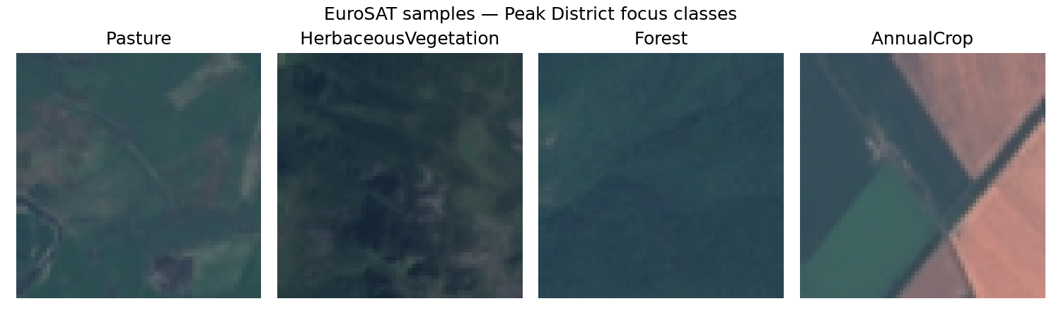
Show one example of each. Save outputs/charts/module1_eurosat_samples.png.

(Compare to subclass codes in the Taylor schema when you open pdnpa/cnn-land-cover.)

— Andy

Why this matters

Professional land mapping almost always starts with public or client-supplied imagery, not arrays you drew in numpy. EuroSAT is a standard teaching dataset because the tiles are small, labelled and free — close enough to the Peak District problem that the skills transfer.

What you'll learn

• How to load EuroSAT via TensorFlow Datasets
• How satellite "levels" relate to grass, forest and crops
• Why 64×64 patches are both convenient and limiting

Step 1 — Create the notebook

notebooks/module1_eurosat.ipynb

Section 1 — Load EuroSAT

Question

Can we download a real labelled satellite dataset in a few lines?

Note: TensorFlow Datasets often fails with HTTP 403 on the old EuroSAT URL. Use eurosat_loader.py from the starter kit (Zenodo mirror).

Code — recommended (Zenodo via starter kit)

Copy eurosat_loader.py into your cnn201 folder, then:

import numpy as np
import matplotlib.pyplot as plt
from eurosat_loader import load_eurosat

X_train, y_train, X_test, y_test, CLASS_NAMES = load_eurosat(
    test_fraction=0.15, seed=0
)

print("Train:", X_train.shape, "Test:", X_test.shape)
print("Classes:", CLASS_NAMES)

Code — alternative (TensorFlow Datasets, if it works on your machine)

import numpy as np
import matplotlib.pyplot as plt
import tensorflow as tf
import tensorflow_datasets as tfds

(ds_train, ds_test), ds_info = tfds.load(
    "eurosat",
    split=["train[:85%]", "train[85%:]"],
    as_supervised=True,
    with_info=True,
    batch_size=-1,
)
X_train = ds_train[0].numpy()
y_train = ds_train[1].numpy()
X_test = ds_test[0].numpy()
y_test = ds_test[1].numpy()
CLASS_NAMES = ds_info.features["label"].names

print("Train:", X_train.shape, "Test:", X_test.shape)
print("Classes:", CLASS_NAMES)

If this raises DownloadError or 403, switch to eurosat_loader.py above.

What the code does

EuroSAT ships one label per 64×64 RGB tile. We hold out 15% as a test set before any filtering — you will refine splits in Module 2.

Section 2 — Filter to Peak District–relevant classes

Code

CLASS_NAMES = ds_info.features["label"].names  # skip this line if you used eurosat_loader
FOCUS = ["Pasture", "HerbaceousVegetation", "Forest", "AnnualCrop"]
FOCUS_IDS = [CLASS_NAMES.index(c) for c in FOCUS]

def filter_classes(X, y, ids):
    mask = np.isin(y, ids)
    Xf, yf = X[mask], y[mask]
    # Remap labels to 0..3 for simpler training later
    remap = {old: new for new, old in enumerate(ids)}
    yf = np.array([remap[v] for v in yf])
    return Xf, yf

X_train, y_train = filter_classes(X_train, y_train, FOCUS_IDS)
X_test, y_test = filter_classes(X_test, y_test, FOCUS_IDS)

for i, name in enumerate(FOCUS):
    print(f"{i} {name:25s} train count: {(y_train == i).sum()}")

What the code does

We discard highways, rivers, cities and so on — they are not part of this Peak District grazing map. Labels become 0–3 instead of EuroSAT's full 0–9 range.

Section 3 — Contact sheet

Code

fig, axes = plt.subplots(1, 4, figsize=(10, 3))
for i, name in enumerate(FOCUS):
    idx = np.where(y_train == i)[0][0]
    axes[i].imshow(X_train[idx])
    axes[i].set_title(name)
    axes[i].axis("off")
plt.suptitle("EuroSAT samples — Peak District focus classes")
plt.tight_layout()
plt.savefig("../outputs/charts/module1_eurosat_samples.png", dpi=150)
plt.show()

What the code does

Look carefully: Pasture is often smoother and brighter green. HerbaceousVegetation can look patchier — closer to rough moor. Forest is darker and more textured. AnnualCrop may show field geometry. These are clues a CNN can learn — and cases where even humans disagree.

Expected result: four distinct 64×64 tiles. Compare with the sample contact sheet.

Reflection questions

• Could you label these four classes confidently without a legend?
• Why might a Peak District ranger care about Pasture vs HerbaceousVegetation separately?
• What is missing compared to a full park map (patch size, geography, season)?

Manager feedback

From: Andy Ipping

Good. Real tiles are messier than our synthetic ones — shadows, mixed pixels, odd colours. That is normal.

Tomorrow: split carefully and learn to read mistakes from a confusion matrix, not just a single accuracy number.

— Andy

AQA Mathematics links

• Sampling — train vs test as two samples from the same population
• Frequency tables — class counts before training

Beyond A-Level

Search for Sentinel-2 bands. Operational Peak District maps often use near-infrared, not just RGB, to separate vegetation types.

Module 2 — Split & Evaluate Honestly

Manager email

From: Andy Ipping
Subject: No cheating — validation before you celebrate

A client once showed me 99% accuracy. The model had memorised the filenames. We do not do that here.

1. Scale pixels to 0–1.
2. Keep your test set untouched until the end.
3. Create a validation split from training data for tuning.
4. Train the same tiny CNN architecture from CNN 101 and report test accuracy once.

Save a confusion matrix to outputs/charts/module2_confusion.png.

— Andy

Why this matters

Data leakage — letting test information influence training — is one of the most common mistakes in junior ML work. Land-cover projects are especially seductive because high accuracy looks impressive on slides but means nothing if the model fails on next year's imagery.

What you'll learn

• Train / validation / test roles
• Normalising pixel values
• Reading a confusion matrix row by row

Step 1 — Create the notebook

notebooks/module2_evaluation.ipynb

Reuse X_train, y_train, X_test, y_test, and FOCUS from Module 1, or reload and filter EuroSAT the same way.

Section 1 — Scale and split validation

You now have three data roles. Read this before running the code:

EuroSAT (all tiles)
├── X_test, y_test     ← 15% held back on day one — touch once at the end
└── X_train, y_train   ← the other 85%
    ├── X_tr, y_tr     ← 80% of this — model learns here
    └── X_val, y_val   ← 20% of this — check while training

In the code below, test_size=0.8 means 80% of the training pool goes to X_tr and 20% becomes validation — not an 80% test set.

Code

import numpy as np
from sklearn.model_selection import train_test_split
import tensorflow as tf
from tensorflow import keras

# Baseline CNN: scale pixels to 0–1
X = X_train.astype("float32") / 255.0
X_tr, X_val, y_tr, y_val = train_test_split(
    X, y_train, test_size=0.2, stratify=y_train, random_state=0
)
X_test_scaled = X_test.astype("float32") / 255.0

X_tr.shape, X_val.shape, X_test_scaled.shape

Section 2 — Baseline CNN (same family as CNN 101)

Code

model = keras.Sequential([
    keras.layers.Conv2D(32, 3, activation="relu", input_shape=(64, 64, 3)),
    keras.layers.MaxPooling2D(2),
    keras.layers.Conv2D(64, 3, activation="relu"),
    keras.layers.MaxPooling2D(2),
    keras.layers.Flatten(),
    keras.layers.Dense(64, activation="relu"),
    keras.layers.Dense(4, activation="softmax"),
])
model.compile(
    optimizer="adam",
    loss="sparse_categorical_crossentropy",
    metrics=["accuracy"],
)
history = model.fit(
    X_tr, y_tr,
    validation_data=(X_val, y_val),
    epochs=15,
    batch_size=64,
    verbose=1,
)
test_loss, test_acc = model.evaluate(X_test_scaled, y_test, verbose=0)
print(f"Test accuracy (one shot): {test_acc:.1%}")

Note validation accuracy while training. If train accuracy rises but validation flatlines, you are overfitting — the model memorises training tiles instead of learning general patterns.

Section 3 — Confusion matrix

Code

import matplotlib.pyplot as plt
from sklearn.metrics import ConfusionMatrixDisplay, confusion_matrix

y_pred = model.predict(X_test_scaled, verbose=0).argmax(axis=1)
cm = confusion_matrix(y_test, y_pred)

fig, ax = plt.subplots(figsize=(6, 5))
disp = ConfusionMatrixDisplay(cm, display_labels=FOCUS)
disp.plot(ax=ax, cmap="Blues", xticks_rotation=45, values_format="d")
plt.title("Baseline CNN — test set confusion")
plt.tight_layout()
plt.savefig("../outputs/charts/module2_confusion.png", dpi=150)
plt.show()

What the code does

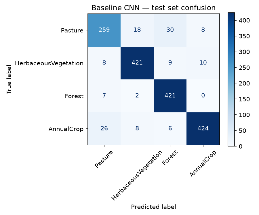
Rows = true class, columns = predicted. Large off-diagonal counts tell you which pairs confuse the model — e.g. Pasture vs HerbaceousVegetation is a common struggle because both are green from above.

Expected result: most counts on the diagonal; largest off-diagonal block often Pasture ↔ HerbaceousVegetation or HerbaceousVegetation ↔ Forest. See the sample confusion matrix.

Your written task

report/module2_evaluation_note.md (150–200 words):

1. Your test accuracy.
2. One pair of classes the model confuses — why might that happen visually?
3. One reason test accuracy might overstate real Peak District performance.

Manager feedback

From: Andy Ipping

Solid baseline. If Pasture and HerbaceousVegetation swap places, rangers might still find the map useful — but we must say so in the brief.

Next: augmentation, the cheapest way to teach a model "this field looks different under cloud shadow."

— Andy

Module 3 — Augmentation for Aerial Photos

Manager email

From: Andy Ipping
Subject: Same field, different day — augment your training set

We cannot reshoot the Peak District every time lighting changes. We simulate variation: flips, small rotations, brightness shifts.

Add a Keras augmentation layer to your pipeline, retrain, and tell me whether validation accuracy improved. Save learning curves to outputs/charts/module3_augmentation.png.

— Andy

Why this matters

Data augmentation artificially expands training data by applying realistic transforms. For aerial imagery, flips and rotations are often safe (there is no "up" in a map tile). Brightness shifts mimic sun angle and cloud cover.

Honest reporting: Augmentation will not always beat your Module 2 baseline. Your job is to describe what happened — flat or lower validation curves are still a valid result worth explaining to Andy.

Step 1 — Create the notebook

notebooks/module3_augmentation.ipynb

Section 1 — Augmentation layer

Code

import tensorflow as tf
from tensorflow import keras

data_augmentation = keras.Sequential([
    keras.layers.RandomFlip("horizontal_and_vertical"),
    keras.layers.RandomRotation(0.1),
    keras.layers.RandomContrast(0.1),
])

inputs = keras.Input(shape=(64, 64, 3))
x = data_augmentation(inputs)
x = keras.layers.Conv2D(32, 3, activation="relu")(x)
x = keras.layers.MaxPooling2D(2)(x)
x = keras.layers.Conv2D(64, 3, activation="relu")(x)
x = keras.layers.MaxPooling2D(2)(x)
x = keras.layers.Flatten()(x)
x = keras.layers.Dense(64, activation="relu")(x)
outputs = keras.layers.Dense(4, activation="softmax")(x)
model_aug = keras.Model(inputs, outputs)
model_aug.compile(
    optimizer="adam",
    loss="sparse_categorical_crossentropy",
    metrics=["accuracy"],
)

What the code does

Augmentation runs only during training — each epoch sees slightly different versions of the same tiles. Test images are never augmented.

Section 2 — Train and compare

Run in the same notebook session as Module 2 so history (baseline validation curve) is still in memory. If you restarted, re-run Module 2 Section 2 first.

Code

hist_aug = model_aug.fit(
    X_tr, y_tr,
    validation_data=(X_val, y_val),
    epochs=15,
    batch_size=64,
    verbose=1,
)

plt.figure(figsize=(8, 4))
plt.plot(history.history["val_accuracy"], label="baseline (Module 2)")
plt.plot(hist_aug.history["val_accuracy"], label="with augmentation")
plt.xlabel("Epoch")
plt.ylabel("Validation accuracy")
plt.title("Did augmentation help?")
plt.legend()
plt.tight_layout()
plt.savefig("../outputs/charts/module3_augmentation.png", dpi=150)
plt.show()

test_loss, test_acc_aug = model_aug.evaluate(X_test_scaled, y_test, verbose=0)
print(f"Test accuracy with augmentation: {test_acc_aug:.1%}")

Section 3 — Visualise augmented tiles

Code

fig, axes = plt.subplots(2, 5, figsize=(12, 5))
sample = X_tr[:1]
for ax in axes.flat:
    aug = data_augmentation(sample, training=True)
    ax.imshow(aug[0].numpy())
    ax.axis("off")
plt.suptitle("One pasture tile — random augmentations")
plt.tight_layout()
plt.show()

Reflection questions

• Did augmentation help your validation curve? If not, why might 15 epochs be too few or too many?
• Would vertical flips always be realistic for aerial photos with shadows?
• What augmentations would not make sense (e.g. turning a river upside-down while keeping its label)?

Manager feedback

From: Andy Ipping

Augmentation is not magic — it cannot fix wrong labels. But it often stops models from latching onto "this exact shade of green."

Tomorrow: transfer learning — stand on a network that already learned edges and textures from millions of photos.

— Andy

Module 4 — Transfer Learning

Manager email

From: Andy Ipping
Subject: Borrow a backbone — MobileNetV2

Training a deep CNN from scratch on 20,000 small tiles works, but it is slow and hungry for data. We will use MobileNetV2, pre-trained on ImageNet, freeze its early layers, and retrain only the top for our four land classes.

Beat your Module 2 baseline on the test set if you can. Save the model to models/eurosat_peaks.keras.

— Andy

Why this matters

Transfer learning reuses features learned on a large general dataset. Early CNN layers detect edges and textures everywhere — grass, faces, cars. You only retrain the head for Pasture vs Forest. This is standard practice in operational remote sensing.

Step 1 — Create the notebook

notebooks/module4_transfer.ipynb

Section 1 — Build the model

Code

import tensorflow as tf
from tensorflow import keras

IMG_SIZE = 64

base = keras.applications.MobileNetV2(
    input_shape=(IMG_SIZE, IMG_SIZE, 3),
    include_top=False,
    weights="imagenet",
)
base.trainable = False  # freeze pre-trained weights

inputs = keras.Input(shape=(IMG_SIZE, IMG_SIZE, 3))
x = keras.applications.mobilenet_v2.preprocess_input(inputs)
x = base(x, training=False)
x = keras.layers.GlobalAveragePooling2D()(x)
x = keras.layers.Dropout(0.3)(x)
outputs = keras.layers.Dense(4, activation="softmax")(x)
model_tl = keras.Model(inputs, outputs)

model_tl.compile(
    optimizer=keras.optimizers.Adam(learning_rate=1e-3),
    loss="sparse_categorical_crossentropy",
    metrics=["accuracy"],
)
model_tl.summary()

What the code does

MobileNetV2 expects a specific input scaling — preprocess_input handles that. GlobalAveragePooling2D collapses spatial features into one vector per image. Dropout reduces overfitting on the small head.

Critical — do not skip: preprocess_input expects pixel values in 0–255, not 0–1. If you already divided by 255 for the baseline CNN, create separate arrays for transfer learning (X_tr * 255.0, etc.). Mixing 0–1 data with preprocess_input silently destroys accuracy (~50% instead of ~90%).

Section 2 — Train the head

Code

# MobileNet preprocess_input expects 0–255 (not the 0–1 arrays from Module 2)
X_tr_tl = X_tr * 255.0
X_val_tl = X_val * 255.0
X_test_tl = X_test_scaled * 255.0

history_tl = model_tl.fit(
    X_tr_tl, y_tr,
    validation_data=(X_val_tl, y_val),
    epochs=10,
    batch_size=64,
    verbose=1,
)

test_loss, test_acc_tl = model_tl.evaluate(X_test_tl, y_test, verbose=0)
print(f"Transfer learning test accuracy: {test_acc_tl:.1%}")

model_tl.save("../models/eurosat_peaks.keras")

First MobileNetV2 download is ~9 MB via Keras.

Section 3 — Optional fine-tuning

If validation accuracy plateaued early, unfreeze the last few layers:

Code

base.trainable = True
for layer in base.layers[:-20]:
    layer.trainable = False

model_tl.compile(
    optimizer=keras.optimizers.Adam(learning_rate=1e-5),
    loss="sparse_categorical_crossentropy",
    metrics=["accuracy"],
)
model_tl.fit(X_tr_tl, y_tr, validation_data=(X_val_tl, y_val), epochs=5, batch_size=64)

Use a much smaller learning rate when fine-tuning — you are nudging pre-trained weights, not rewriting them.

Reflection questions

• Why freeze the base first instead of training everything immediately?
• ImageNet contains cats and cars, not moorland. Why does transfer still help?
• What would you check before deploying this model on 2026 imagery?

Manager feedback

From: Andy Ipping

This is the workflow our production team uses — backbone plus small head, honest test score, saved model file.

Friday: package results for the park office. They do not want code; they want a map they can trust and limitations they can explain to councillors.

— Andy

Beyond A-Level

Look up fine-tuning learning rates and domain shift — when satellite sensors or seasons change enough that a model needs retraining.

Module 5 — Professional Project

Manager email

From: Andy Ipping
Subject: Brief for colleagues — same template as Landscape Recovery reviews

Deliverables:

1. notebooks/module5_project.ipynb — final test-set evaluation
2. outputs/charts/module5_confusion_and_samples.png
3. report/module5_park_brief.md — 400–500 words for non-technical colleagues (rangers, ecologists, Landscape Recovery partners)

Structure: question → method → accuracy → main confusions → limitations → recommendation. State clearly this is EuroSAT practice, not an operational map — this exercise uses EuroSAT unless you also ran pdnpa/cnn-land-cover.

— Andy

Why this matters

Computer vision engineers spend as much time communicating uncertainty as training models. A 85% accurate map can be actionable if errors cluster in harmless places — or useless if it mislabels SSSI woodland as pasture.

Section 1 — Wrong vs right gallery

Ensure X_test_tl = X_test_scaled * 255.0 exists from Module 4 before running.

Code

import numpy as np
import matplotlib.pyplot as plt
from tensorflow import keras
from sklearn.metrics import confusion_matrix

model = keras.models.load_model("../models/eurosat_peaks.keras")
y_pred = model.predict(X_test_tl, verbose=0).argmax(axis=1)

correct = np.where(y_pred == y_test)[0]
wrong = np.where(y_pred != y_test)[0]

fig, axes = plt.subplots(2, 4, figsize=(12, 6))
for ax, idx in zip(axes[0], correct[:4]):
    ax.imshow(X_test[idx])
    ax.set_title(f"OK: {FOCUS[y_test[idx]]}")
    ax.axis("off")
for ax, idx in zip(axes[1], wrong[:4]):
    ax.imshow(X_test[idx])
    ax.set_title(f"Miss: true {FOCUS[y_test[idx]]}\npred {FOCUS[y_pred[idx]]}")
    ax.axis("off")
plt.suptitle("Correct vs incorrect test tiles")
plt.tight_layout()
plt.savefig("../outputs/charts/module5_confusion_and_samples.png", dpi=150)
plt.show()

Section 2 — Brief outline

Your report/module5_park_brief.md should answer:

1. What we mapped — four land classes from satellite tiles.
2. How — EuroSAT, CNN with transfer learning, train/test split.
3. Accuracy — quote test accuracy; name the worst confusion pair.
4. Limitations — 64×64 patches, not full Peak District; European tiles, not necessarily Derbyshire; no ground survey; season unknown.
5. Recommendation — e.g. "Use as draft map only; verify pasture boundaries on foot before grazing decisions."

Reflection questions

• Would you sign this brief if you knew rangers would graze livestock from it?
• Which limitation matters most — patch size, geography, or season?
• What ground-truth check would you propose (sample fields to visit)?

Manager feedback

From: Andy Ipping

If I can read your limitations paragraph and still see a path to a useful product, you think like a consultant — not a Kaggle competitor.

CNN 301 is unguided. Same domain, your question, your deliverable.

— Andy

Module 6 — What You Have Learned

By the end of CNN 201, you will be able to:

1. load public imagery and relate classes to habitat groups from the published schema;
2. split train, validation and test sets and read confusion matrices honestly;
3. apply augmentation suited to multi-date aerial surveys;
4. fine-tune a pre-trained CNN backbone;
5. write a land-cover brief suitable for rangers and Landscape Recovery partners.

If you enjoyed real imagery, model tuning and writing for decision-makers, continue to Computer Vision Developer 301 for an open project of your own.

Analyst path: Computer Vision Analyst 301.

Next steps: Computer Vision Developer 301 when you are ready to choose the question yourself.