Quantitative Finance · Level 101
Quant 101 — Could I Be a Quant?
Shadow a junior quant at Aurora Capital — from market data to strategy backtests and a client research note.
Quantitative Finance · Level 101
Quant 101 — Could I Be a Quant?
Shadow a junior quant at Aurora Capital — from market data to strategy backtests and a client research note.
Quant 101 — Could I Be a Quant?
Prerequisite: Data Science 101.
This course assumes you can already use VS Code, Jupyter Notebooks, Python, pandas and matplotlib. We won't reteach those. Instead, you'll discover how quantitative analysts use those tools to make investment decisions.
You have joined Aurora Capital, a mid-sized London asset manager. Your manager is Elena Vasquez, a portfolio manager who relies on the quant team to turn market data into decisions.
Over five modules you will do real junior-quant work:
- Understand what quants do and whether the career appeals to you.
- Download market data and measure risk the way traders do.
- Test a simple trading strategy and ask whether it is genuine or luck.
- Compare portfolios under uncertainty.
- Write a short research note for Elena on a live question about NVIDIA and Apple.
Sample student outputs: Worked examples. Your charts should look broadly similar (daily returns, moving averages, Monte Carlo, earnings bars) — not identical.
The mindset to keep throughout:
price → return → risk → decision
Before you start — create your project folder
Open File Explorer (or Finder on Mac).
Create a folder called quant101 inside your existing coding folder (the
same parent folder you used for Data Science).
Inside quant101, create:
Open VS Code. Choose File → Open Folder and open quant101.
You will save downloaded Yahoo Finance CSVs in data/, notebooks in
notebooks/, charts in outputs/charts/, and short written answers in
report/.
Tools
- VS Code
- Jupyter Notebook
- Python
- pandas
- matplotlib
- Yahoo Finance (download historical CSVs manually)
If you need a package you have not installed yet:
pip install pandas matplotlib jupyter ipykernelModule 1 — What is a Quant?
Manager email
From: Elena Vasquez
Subject: Welcome to Aurora CapitalWelcome aboard. Before I give you any market data, I need to know whether you understand what a quant actually does — and whether you find that kind of work interesting.
This week, read about three firms: Jane Street, Citadel and Man Group. All hire quantitative people in the UK. Check each firm's careers page and its internships section — the internship pages often explain what the work is really like. Then send me a one-page note answering:
- What does a quant do day to day?
- Why do these firms pay so well?
- Which firm sounds most interesting to you, and why?
No Python required today. Think like an analyst, not a programmer.
— Elena
Why this matters
Portfolio managers do not hire quants because they enjoy spreadsheets. They hire quants because markets are uncertain and expensive mistakes are possible.
A quant's job is to:
- turn prices into measurable risk;
- test ideas before real money is deployed;
- explain results clearly to non-specialists.
If you dislike careful reasoning under uncertainty, you will not enjoy this career — even if you are good at Python.
What you'll learn
- What a quantitative analyst does
- The difference between hedge funds, investment banks and asset managers
- What shares are and why people trade them
- Typical UK career paths and graduate salaries
- Whether this style of work feels motivating to you
What is a share?
When you buy a share in Apple, you own a tiny fraction of the company.
If Apple grows profits, investors often pay more for each share — the share price rises. If investors worry about the future, the price can fall even when the company still sells iPhones.
Quants rarely care about the brand story alone. They start with prices and returns — the numbers that move portfolios.
Three types of employer
| Type | Example | Quant work often involves… |
|---|---|---|
| Hedge fund | Citadel | Fast strategies, strict risk limits |
| Market maker / prop trading | Jane Street | Pricing, liquidity, tight feedback loops |
| Asset manager | Man Group | Research for long-term client portfolios |
Aurora Capital is closest to an asset manager: we look after pension and charity money over years, not minutes.
Your tasks
Create a new file:
report/module1_quant_research.md
Answer the following in clear prose (roughly 300–500 words total).
Task 1 — Research three firms
Visit the careers pages of Jane Street, Citadel and Man Group. For each firm, also check its internships section if one exists — many quant employers hire through summer internship programmes rather than straight graduate roles. For example, Jane Street publishes its internship overview at janestreet.com/join-jane-street/internships/.
For each firm, note:
- what the firm says it does;
- one example role that mentions mathematics, programming or research;
- where in the UK it hires;
- whether it offers internships (and what they involve, if so).
Task 2 — Compare graduate pay (roughly)
Search "quant graduate salary UK" and read two recent sources (job boards, BrightNetwork, firm pages). You do not need exact figures — estimate a range and cite your sources.
Task 3 — Explain the premium
In your own words: why might a firm pay a quant graduate more than many other graduate roles? Connect your answer to risk, speed and money under management.
Task 4 — Pick one firm
Which of the three would you most like to learn more about? One honest paragraph — there is no correct answer.
Reflection questions
Add a short section at the bottom of your report:
- Did you enjoy the research, or did you find it tedious?
- Did the salary information change your interest, or not really?
- Did any job description sound exciting? Any sound miserable?
- Do you like the idea of being wrong in public when a model fails?
Manager feedback
From: Elena Vasquez
Good first effort. A few things strong quants always do in week one:
- They distinguish facts from marketing language on careers pages.
- They check internship pages as well as graduate listings — that is often where you learn what day-to-day work actually looks like.
- They notice whether they enjoy hunting for evidence — that matters more than liking maths in abstract.
- They ask who loses money when a model is wrong.
If you felt curious and wanted to dig deeper, that is a good sign. If you were bored unless something flashed on a screen, notice that too.
Tomorrow we look at real prices. Bring your Python environment.
— Elena
AQA Mathematics links
- Statistics — interpreting data and sources critically
- Probability — uncertainty as a core idea in markets
Beyond A-Level
Look up efficient market hypothesis. Do prices already reflect public information? Quants disagree — and that disagreement employs thousands of people.
Module 2 — Markets as Data
Manager email
From: Elena Vasquez
Subject: Four stocks, one question — how risky are they?I am comparing four names for a client mandate:
- NVIDIA (AI infrastructure)
- Apple (consumer technology)
- Shell (energy)
- SPY (a fund tracking the broad US market — our benchmark)
Download two years of daily prices for each. Calculate daily returns, measure volatility, and find the largest one-day move for each name.
For the biggest NVIDIA move: find a news headline from that date and explain the connection in two sentences.
Save one chart I can paste into a client slide deck.
— Elena
Why this matters
Before Aurora buys millions of pounds of a stock, someone on my team answers boring-sounding questions:
- How bumpy has this been day to day?
- Was one company much wilder than the market as a whole?
- Did a single news day dominate the risk?
That is not "prediction" yet. It is measurement — the step quants never skip.
What you'll learn
- Download historical prices from Yahoo Finance
- Load share price CSVs with pandas
- Calculate daily returns
- Measure volatility (standard deviation of returns)
- Identify extreme moves and connect them to real events
Step 1 — Download the data from Yahoo Finance
For each ticker below, download two years of daily historical prices with Adjusted Close included.
| Company | Yahoo Finance ticker |
|---|---|
| NVIDIA | NVDA |
| Apple | AAPL |
| Shell | SHEL |
| S&P 500 ETF | SPY |
How to download (repeat for each ticker):
- Go to https://finance.yahoo.com.
- Search the ticker (e.g.
NVDA). - Click Historical Data.
- Set Time Period to 2 years.
- Click Apply.
- Click Download.
- Save the file into
quant101/data/asNVDA.csv,AAPL.csv,SHEL.csv,SPY.csv.
Open one CSV in Excel briefly. Confirm columns include Date and Adj Close (or Close if Adj Close is missing — note which you used in your notebook).
Step 2 — Create the notebook
In VS Code, create:
notebooks/module2_markets_as_data.ipynb
Select your Python kernel (same as Data Science).
Section 1 — Load one price file
Question
Can pandas read NVIDIA's price history?
Code
import pandas as pd

path = "../data/NVDA.csv"
nvda = pd.read_csv(path)
nvda.head()
What the code does
pd.read_csv loads the downloaded Yahoo file. head() shows the first rows so
you can check dates and prices look sensible.
If your CSV uses a different date column name, adjust later steps accordingly.
Section 2 — Keep date and adjusted close
Question
Which columns do we actually need?
Code
nvda["Date"] = pd.to_datetime(nvda["Date"])
price_col = "Adj Close" if "Adj Close" in nvda.columns else "Close"

prices = nvda[["Date", price_col]].rename(columns={price_col: "price"})
prices = prices.sort_values("Date").reset_index(drop=True)
prices.head()
What the code does
We convert Date to proper datetime objects, keep one price column, sort
oldest → newest, and reset the row index.
Adjusted close accounts for splits and dividends. Quants prefer it when available.
Section 3 — Daily returns
Question
How much did NVIDIA move each day?
Code
prices["return"] = prices["price"].pct_change()
prices[["Date", "price", "return"]].tail()
What the code does
pct_change() computes the percentage change from one row to the next:
The first row is blank — there is no previous day yet.
Section 4 — Volatility
Question
How bumpy was NVIDIA day to day?
Code
daily_vol = prices["return"].std()
annualised_vol = daily_vol * (252 ** 0.5)

daily_vol, annualised_vol
What the code does
std() is the standard deviation of daily returns — a standard volatility
measure.
Multiplying by scales up from daily to a rough annualised figure (252 ≈ trading days per year). Different firms use slightly different conventions — the idea matters more than the exact constant.
Section 5 — Largest one-day move
Question
Which single day moved most?
Code
worst = prices.loc[prices["return"].idxmin()]
best = prices.loc[prices["return"].idxmax()]

worst, best
What the code does
idxmin() and idxmax() find the row indices of the worst and best daily
returns. loc pulls the full row including the date.
Search that date on a news site. Write two sentences in your notebook explaining what happened.
You will do this for NVIDIA in Elena's summary below. For Shell, prefer an oil or energy headline (OPEC, crude prices, geopolitics) — Shell is in the download so you can practise linking an energy name to the commodity story, not only AI/tech news.
Section 6 — Compare all four names
Question
Can we repeat this for Apple, Shell and the market benchmark?
Code
tickers = {
    "NVDA": "../data/NVDA.csv",
    "AAPL": "../data/AAPL.csv",
    "SHEL": "../data/SHEL.csv",
    "SPY": "../data/SPY.csv",
}

rows = []

for name, file_path in tickers.items():
    df = pd.read_csv(file_path)
    df["Date"] = pd.to_datetime(df["Date"])
    col = "Adj Close" if "Adj Close" in df.columns else "Close"
    df = df.sort_values("Date")
    rets = df[col].pct_change()
    rows.append({
        "ticker": name,
        "daily_vol": rets.std(),
        "annualised_vol": rets.std() * (252 ** 0.5),
        "worst_day": rets.min(),
        "best_day": rets.max(),
    })

summary = pd.DataFrame(rows)
summary
What the code does
We loop over each file, compute the same statistics, and collect results in a table. This is exactly the kind of "boring" reusable code quants write once and run every Monday.
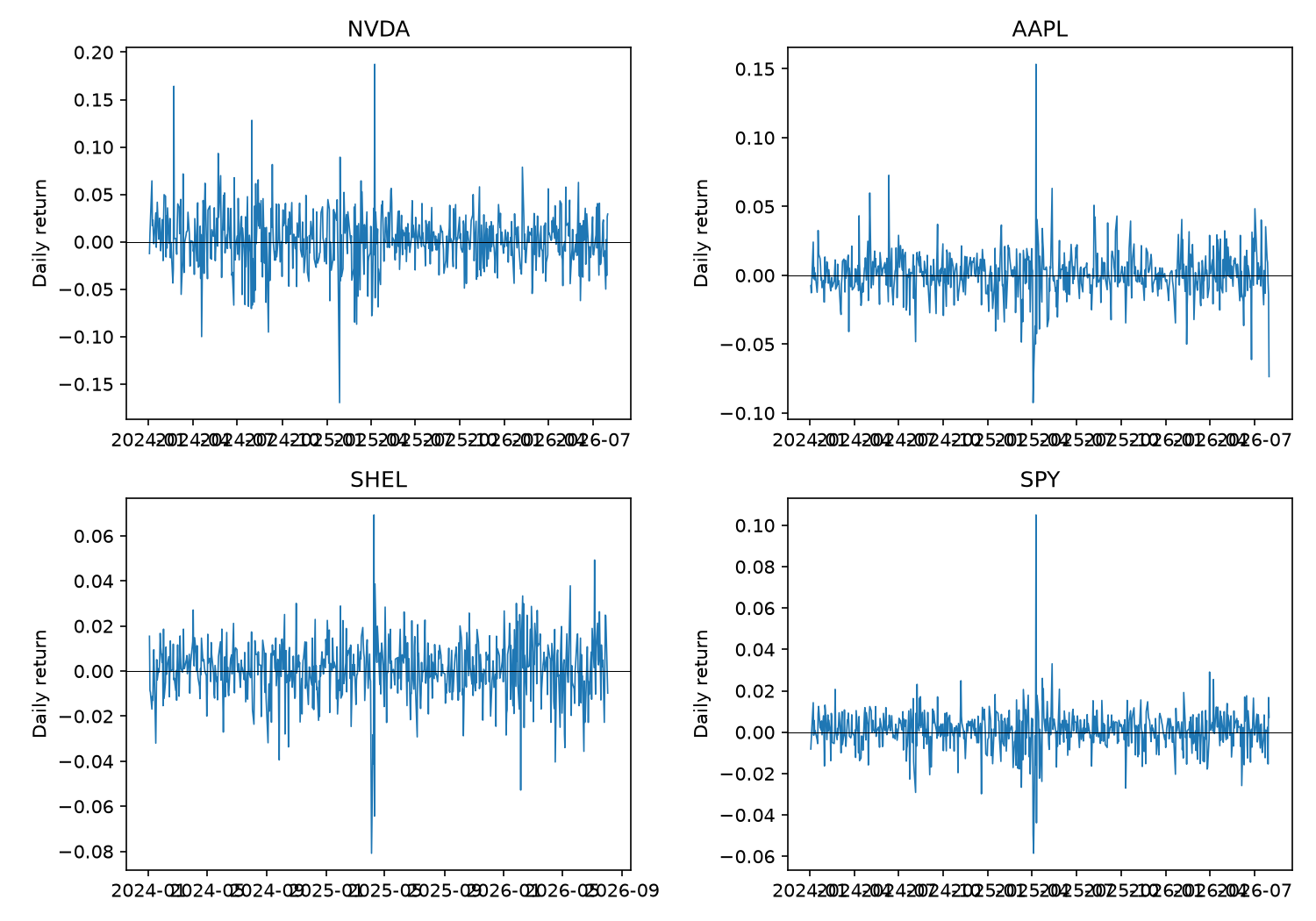
Section 7 — Chart daily returns
Question
Can Elena see the bumpiness visually?
Code
import matplotlib.pyplot as plt

fig, axes = plt.subplots(2, 2, figsize=(10, 7), sharex=False)
axes = axes.flatten()

for ax, (name, file_path) in zip(axes, tickers.items()):
    df = pd.read_csv(file_path)
    df["Date"] = pd.to_datetime(df["Date"])
    col = "Adj Close" if "Adj Close" in df.columns else "Close"
    df = df.sort_values("Date")
    df["return"] = df[col].pct_change()
    ax.plot(df["Date"], df["return"], linewidth=0.8)
    ax.set_title(name)
    ax.set_ylabel("Daily return")
    ax.axhline(0, color="black", linewidth=0.5)

plt.tight_layout()
plt.savefig("../outputs/charts/module2_daily_returns.png", dpi=150)
plt.show()
What the code does
Four small charts let you compare how wildly each name moved day to day. The saved PNG is what Elena meant by "client slide deck".
Compare with the sample daily-returns chart.
Section 8 — Write Elena's summary
Add a markdown cell answering:
- Which ticker was most volatile?
- Was NVIDIA more volatile than SPY? By roughly how much?
- For NVIDIA's worst day: what news headline did you find?
- For Shell's worst day: what oil or energy headline fits the move?
- Would you describe Shell as a "quiet" stock compared with NVIDIA? Use numbers.
Reflection questions
- Did you enjoy hunting for the news story behind a price move?
- Did any result surprise you?
- Would you trust a single volatility number without plotting the data?
Manager feedback
From: Elena Vasquez
Solid work. Two habits to keep:
- Always plot — summary statistics hide weird days.
- Always ask "compared to what?" — NVIDIA alone means little; NVIDIA versus SPY means something.
Next you will test a trading idea. Spoiler: most simple ideas do not work. Learning to check anyway is the job.
— Elena
AQA Mathematics links
- Standard deviation — volatility as applied spread
- Sequences and change — day-to-day percentage changes
Beyond A-Level
Look up log returns . Professionals often use them because they combine cleanly across time. Daily simple returns are fine for this course.
Module 3 — Finding an Edge
Manager email
From: Elena Vasquez
Subject: A simple trend idea — but does it actually work?A junior analyst claims: "When NVIDIA's 20-day average price is above its 50-day average, the trend is up — we should be invested."
Test this moving-average strategy on two years of NVIDIA data. Compare it to buying and holding the stock the entire time.
I do not need a fancy model. I need an honest answer: did the rule beat buy-and-hold? Could the result be luck?
— Elena
Why this matters
Quants spend more time rejecting ideas than celebrating them. A moving average rule takes five minutes to code and five years to properly evaluate. Today you do the five-minute version — and practise scepticism.
What you'll learn
- Compute rolling (moving) averages
- Code a simple rule: in the market when short average > long average
- Backtest naively against buy-and-hold
- Ask whether outperformance could be luck or overfitting
Step 1 — Create the notebook
notebooks/module3_moving_average.ipynb
Section 1 — Load NVIDIA prices
Question
Do we have a clean price series?
Code
import pandas as pd
import matplotlib.pyplot as plt

nvda = pd.read_csv("../data/NVDA.csv")
nvda["Date"] = pd.to_datetime(nvda["Date"])
price_col = "Adj Close" if "Adj Close" in nvda.columns else "Close"

prices = nvda[["Date", price_col]].rename(columns={price_col: "price"})
prices = prices.sort_values("Date").reset_index(drop=True)
prices.head()
What the code does
Same loading pattern as Module 2 — consistency saves debugging time.
Section 2 — Moving averages
Question
Where are the 20-day and 50-day trends?
Code
prices["ma_20"] = prices["price"].rolling(20).mean()
prices["ma_50"] = prices["price"].rolling(50).mean()

prices[["Date", "price", "ma_20", "ma_50"]].tail()
What the code does
rolling(20).mean() computes the average of the last 20 closing prices each
day. The first 19 rows are blank; the first 49 rows lack a 50-day average.
Section 3 — Plot price and averages
Question
Can we see when the short average is above the long average?
Code
plt.figure(figsize=(10, 5))
plt.plot(prices["Date"], prices["price"], label="Price", linewidth=1)
plt.plot(prices["Date"], prices["ma_20"], label="20-day MA")
plt.plot(prices["Date"], prices["ma_50"], label="50-day MA")
plt.legend()
plt.title("NVIDIA price and moving averages")
plt.ylabel("Price")
plt.savefig("../outputs/charts/module3_moving_averages.png", dpi=150)
plt.show()
What the code does
When the blue 20-day line is above the orange 50-day line, the strategy rule says "invested". Visual inspection helps before trusting performance numbers.
Section 4 — Strategy signal
Question
On which days are we "in" the stock?
Code
prices["signal"] = (prices["ma_20"] > prices["ma_50"]).astype(int)
prices["return"] = prices["price"].pct_change()

# Strategy return: earn the stock return only when signal == 1
prices["strategy_return"] = prices["return"] * prices["signal"].shift(1)

prices[["Date", "signal", "return", "strategy_return"]].tail()
What the code does
signal is 1 when the trend rule says invested, 0 otherwise.
We shift the signal by one day so we trade on yesterday's signal using today's return — a simple way to avoid pretending we knew today's price before the market opened.
Section 5 — Compare cumulative performance
Question
Did the strategy beat buy-and-hold?
Code
import numpy as np

backtest = prices.dropna(subset=["ma_50", "return"]).copy()

backtest["buy_hold"] = (1 + backtest["return"]).cumprod()
backtest["strategy"] = (1 + backtest["strategy_return"].fillna(0)).cumprod()

final_buy_hold = backtest["buy_hold"].iloc[-1] - 1
final_strategy = backtest["strategy"].iloc[-1] - 1

final_buy_hold, final_strategy
What the code does
We compound daily returns into a growth factor. Subtract 1 at the end to express total return over the period (e.g. 0.45 means +45%).
If final_strategy > final_buy_hold, the rule beat buy-and-hold in this
sample. That is not proof it will work next year.
Section 6 — Chart the comparison
Question
What would Elena see?
Code
plt.figure(figsize=(10, 5))
plt.plot(backtest["Date"], backtest["buy_hold"], label="Buy and hold")
plt.plot(backtest["Date"], backtest["strategy"], label="MA strategy")
plt.legend()
plt.title("NVIDIA: strategy vs buy-and-hold")
plt.ylabel("Growth of £1")
plt.savefig("../outputs/charts/module3_strategy_vs_buyhold.png", dpi=150)
plt.show()
What the code does
Starting at £1 invested, which path ends higher? The gap is the question Elena cares about.
Section 7 — Could this be luck?
Add a markdown cell discussing:
- Sample size — two years is one market environment (maybe mostly AI boom).
- Multiple testing — if you tried fifty rules, one might win by accident.
- Overfitting — tuning 20 and 50 to look best on past data may not repeat.
You do not need formal statistics here — reason clearly.
Optional extension: change 20 and 50 to 10 and 30. Did performance
change a lot? If small tweaks change everything, be suspicious.
Reflection questions
- Did you want the strategy to win? Did that affect how you interpreted results?
- Would you invest real money based on this notebook alone?
- Do you enjoy the sceptical part as much as the coding part?
Manager feedback
From: Elena Vasquez
If your strategy lost to buy-and-hold, good — that is the normal outcome. The important part is that you measured instead of believed.
Quants who survive learn to kill bad ideas quickly. The ones who blow up fall in love with a backtest.
— Elena
AQA Mathematics links
- Sequences — rolling windows as local averages
- Probability — distinguishing signal from noise
Beyond A-Level
Research Sharpe ratio and transaction costs. Real strategies pay fees every time they switch in and out.
Module 4 — Risk & Decisions
Manager email
From: Elena Vasquez
Subject: Two portfolios — which would you recommend?A charity client must choose between:
- Portfolio A: 100% NVIDIA
- Portfolio B: 50% NVIDIA, 50% SPY
Use two years of data. Show me expected trade-offs and simulate possible one-year outcomes with a simple Monte Carlo model.
Write a recommendation in plain English. No jargon without explanation.
— Elena
Why this matters
Clients do not experience average returns — they experience one realised path. Quants use simulation to explain range of outcomes, not just a headline percentage.
What you'll learn
- Expected value as a weighted average outcome
- Diversification through combining imperfectly correlated assets
- Monte Carlo simulation for simple portfolio paths
- Making and defending a recommendation under uncertainty
Step 1 — Create the notebook
notebooks/module4_risk_and_decisions.ipynb
Section 1 — Load and align NVIDIA and SPY
Question
Can we put both return series on the same dates?
Code
import pandas as pd
import numpy as np
import matplotlib.pyplot as plt

def load_returns(path):
    df = pd.read_csv(path)
    df["Date"] = pd.to_datetime(df["Date"])
    col = "Adj Close" if "Adj Close" in df.columns else "Close"
    df = df.sort_values("Date")
    df["return"] = df[col].pct_change()
    return df[["Date", "return"]]

nvda = load_returns("../data/NVDA.csv").rename(columns={"return": "nvda"})
spy = load_returns("../data/SPY.csv").rename(columns={"return": "spy"})

data = pd.merge(nvda, spy, on="Date", how="inner").dropna()
data.head()
What the code does
merge keeps only dates present in both files so portfolio calculations line
up day by day.
Section 2 — Historical portfolio returns
Question
How did the two portfolios behave in the past?
Code
data["portfolio_a"] = data["nvda"]
data["portfolio_b"] = 0.5 * data["nvda"] + 0.5 * data["spy"]

summary = pd.DataFrame({
    "mean_daily": [data["portfolio_a"].mean(), data["portfolio_b"].mean()],
    "vol_daily": [data["portfolio_a"].std(), data["portfolio_b"].std()],
}, index=["Portfolio A (100% NVDA)", "Portfolio B (50/50)"])

summary
What the code does
Portfolio B is a weighted average of daily returns — a standard beginner assumption (ignoring rebalancing details).
Compare mean (typical direction) and std (bumpiness).
Section 3 — Expected value intuition
Question
What is the expected value of a risky trade?
Suppose a coin flip pays +3% if heads and −2% if tails, each with probability 0.5.
Code
outcomes = np.array([0.03, -0.02])
probs = np.array([0.5, 0.5])

expected = (outcomes * probs).sum()
expected
What the code does
Expected value is the probability-weighted average:
Positive expected value does not guarantee profit on one trial — it describes the long-run average if you could repeat many times.
Add a markdown cell: does Portfolio A or B have higher expected daily return in your sample? Is that enough to choose it?
Section 4 — Correlation and diversification
Question
Do NVIDIA and SPY move together?
Code
correlation = data["nvda"].corr(data["spy"])
correlation
What the code does
Correlation near 1 means they move together; lower correlation means diversification may reduce portfolio volatility without removing all return.
A brief history of Monte Carlo
Before you run the simulation, it helps to know where the name came from — and why quants treat it as serious mathematics, not a gimmick.
Randomness as a tool
In the 1940s, mathematicians working on nuclear weapons at Los Alamos faced a question: neutrons bounce through material in messy, random paths. Writing a clean formula for every possible path was impossible.
Stanislaw Ulam and John von Neumann had an idea: pretend you can watch thousands of neutrons move step by step, flipping a coin at each decision point. Average the results. The name Monte Carlo method was suggested because Ulam's uncle liked gambling at the Monte Carlo casino in Monaco — the link to random chance stuck.
The same logic applies far beyond physics:
When the exact answer is too hard to calculate, simulate many random versions and see what typically happens.
From atoms to portfolios
For decades Monte Carlo lived mainly in physics and engineering. From the 1980s onward, finance adopted it aggressively:
- Pension funds simulate thousands of future market paths to ask: "Will we still have enough money in 30 years?"
- Banks estimate how bad a bad day could get (Value at Risk).
- Option traders simulate stock paths to price complex derivatives.
None of these people are "guessing" in a casual sense. They are applying probability at scale — exactly the kind of mathematics you meet in A-Level, extended to problems no pen-and-paper formula can solve cleanly.
What you are doing today
Your notebook uses a simple version called bootstrap Monte Carlo:
- Take historical daily returns (real data, real uncertainty).
- Randomly resample them to build fake but plausible one-year paths.
- Repeat hundreds or thousands of times.
- Look at the distribution of outcomes — not just the average.
You are not predicting the future. You are answering Elena's client question: "What range of outcomes should we prepare for?" That is Monte Carlo thinking applied to a real decision — the same mindset used in London banks and pension consultancies, with bigger computers and more data.
Section 5 — Monte Carlo simulation
Question
What might one year ahead look like?
We will simulate 252 trading days, sampling randomly from historical daily returns (with replacement). This is a simple bootstrap Monte Carlo — not perfect, but good for building intuition.
Code
np.random.seed(42)
simulations = 1000
days = 252

def simulate_portfolio(daily_returns):
    paths = np.random.choice(daily_returns, size=(simulations, days), replace=True)
    growth = (1 + paths).cumprod(axis=1)
    return growth[:, -1] - 1  # total return each simulation

sim_a = simulate_portfolio(data["portfolio_a"].values)
sim_b = simulate_portfolio(data["portfolio_b"].values)

pd.DataFrame({
    "Portfolio A": pd.Series(sim_a).describe(),
    "Portfolio B": pd.Series(sim_b).describe(),
})
What the code does
Each simulation draws 252 random daily returns from history, compounds them, and records the total one-year return. One thousand paths gives a distribution, not a single guess.
Section 6 — Plot simulated outcomes
Question
Can Elena see the trade-off?
Code
plt.figure(figsize=(8, 4))
plt.boxplot([sim_a, sim_b], tick_labels=["Portfolio A", "Portfolio B"])
plt.ylabel("Simulated 1-year return")
plt.title("Monte Carlo: 1000 simulated one-year outcomes")
plt.savefig("../outputs/charts/module4_monte_carlo.png", dpi=150)
plt.show()
What the code does
The box plot compares typical outcomes and spread. Often A has a higher median but wider whiskers — more upside and more pain.
Section 7 — Your recommendation
Create report/module4_recommendation.md (200–300 words) answering:
- Which portfolio would you recommend to a charity that needs the money in three years?
- What could go wrong with your recommendation?
- What would you want to know about the client before deciding?
Reflection questions
- Did you prefer the analytic numbers or writing the recommendation?
- Does simulating outcomes feel reassuring or unsettling?
- Would you rather explain risk to a client or optimise a model alone?
Manager feedback
From: Elena Vasquez
Strong analysts connect numbers to who suffers if we are wrong. Charity mandates often prioritise not blowing up over maximising expected return.
If you recommended Portfolio A without mentioning downside paths, revise your thinking. If you recommended B but could not explain why diversification helped, revise that too.
— Elena
AQA Mathematics links
- Expected value — weighted mean outcome
- Variance and spread — risk as dispersion
- Correlation — structure in paired data
Beyond A-Level
Look up Value at Risk (VaR) and drawdown. Clients often ask: "How bad could a bad year get?"
Module 5 — Final Project
Manager email
From: Elena Vasquez
Subject: Research note — earnings day volatilityBefore our NVIDIA holding review, I want a short research note:
Does NVIDIA tend to move more on earnings days than Apple?
Use daily data you already have plus the earnings dates below. Compare the average absolute daily return on earnings days versus ordinary days.
Deliverables:
- Notebook with calculations
- One chart
- A 400-word note in
report/module5_earnings_note.md— Elena
Why this matters
Earnings announcements release information investors re-price quickly. If a stock jumps more on those days, options traders, risk managers and portfolio managers care — it affects position sizing and expectations.
This is a miniature version of a real desk request: specific question, clean measurement, honest limitations.
Earnings dates to use
These are the day after the US market close earnings announcements (when the daily return in Yahoo data reflects the reaction):
NVIDIA (NVDA)
| Date |
|---|
| 2024-02-22 |
| 2024-05-23 |
| 2024-08-29 |
| 2024-11-21 |
| 2025-02-27 |
Apple (AAPL)
| Date |
|---|
| 2024-02-02 |
| 2024-05-03 |
| 2024-08-02 |
| 2024-11-01 |
| 2025-01-31 |
If your downloaded data does not include 2025 dates, use only the 2024 rows and say so in your limitations section.
Step 1 — Create the notebook
notebooks/module5_earnings_project.ipynb
Section 1 — Load returns for both stocks
Question
Are returns ready to compare?
Code
import pandas as pd
import numpy as np
import matplotlib.pyplot as plt

def load_returns(path):
    df = pd.read_csv(path)
    df["Date"] = pd.to_datetime(df["Date"])
    col = "Adj Close" if "Adj Close" in df.columns else "Close"
    df = df.sort_values("Date")
    df["return"] = df[col].pct_change()
    return df[["Date", "return"]].dropna()

nvda = load_returns("../data/NVDA.csv")
aapl = load_returns("../data/AAPL.csv")

nvda.head()
Section 2 — Flag earnings days
Question
Which rows are earnings reaction days?
Code
nvda_earnings = pd.to_datetime([
    "2024-02-22", "2024-05-23", "2024-08-29", "2024-11-21", "2025-02-27",
])
aapl_earnings = pd.to_datetime([
    "2024-02-02", "2024-05-03", "2024-08-02", "2024-11-01", "2025-01-31",
])

nvda["abs_return"] = nvda["return"].abs()
nvda["is_earnings"] = nvda["Date"].isin(nvda_earnings)

aapl["abs_return"] = aapl["return"].abs()
aapl["is_earnings"] = aapl["Date"].isin(aapl_earnings)

nvda[nvda["is_earnings"]][["Date", "return", "abs_return"]]
What the code does
We use absolute return to measure size of move regardless of direction — a −8% drop counts as 8%.
Section 3 — Compare averages
Question
Who moves more on earnings days?
Code
def compare_earnings(df, name):
    earnings = df.loc[df["is_earnings"], "abs_return"].mean()
    normal = df.loc[~df["is_earnings"], "abs_return"].mean()
    return pd.Series({"ticker": name, "earnings_day": earnings, "normal_day": normal})

results = pd.DataFrame([
    compare_earnings(nvda, "NVDA"),
    compare_earnings(aapl, "AAPL"),
])
results
What the code does
Compare mean absolute return on flagged days versus all other days in your sample.
Section 4 — Chart
Question
Can Elena see the pattern?
Code
labels = ["NVDA earnings", "NVDA normal", "AAPL earnings", "AAPL normal"]
values = [
    results.loc[0, "earnings_day"],
    results.loc[0, "normal_day"],
    results.loc[1, "earnings_day"],
    results.loc[1, "normal_day"],
]

plt.figure(figsize=(8, 4))
plt.bar(labels, values)
plt.ylabel("Mean absolute daily return")
plt.title("Earnings days vs normal days")
plt.xticks(rotation=15)
plt.tight_layout()
plt.savefig("../outputs/charts/module5_earnings_volatility.png", dpi=150)
plt.show()
Section 5 — Write the research note
Create report/module5_earnings_note.md with this structure:
- Question — restate Elena's request in one sentence.
- Method — data source, date range, how you flagged earnings days.
- Results — quote your four means; state who moves more on earnings.
- Limitations — small number of earnings days; one market regime; no options data; dates approximate.
- Recommendation — should Aurora expect more earnings-day noise in NVIDIA than Apple? One paragraph.
A sample note is on Worked examples.
Reflection questions
- Did this feel like a job task or a school exercise?
- Which part would you want to do again — coding, charting, or writing?
- After five modules, do you want to learn more about this career?
Manager feedback
From: Elena Vasquez
If I received this note on my desk, I would read the limitations section first — that tells me whether I can trust the analyst.
You are not a quant yet. But you now think in returns, scepticism, and client context. That is the right direction.
If you want to go further, Quant 201 goes deeper into statistics, derivatives and building your own strategy properly.
— Elena
AQA Mathematics links
- Averages and spread — comparing groups of returns
- Probability — events (earnings) and unusual outcomes
Beyond A-Level
Look up implied volatility around earnings. Options markets often predict large moves before announcements — a whole sub-field quants work in.
Module 6 — What You Have Learned
By the end of Quant 101, you have learned to:
- research what quants do and whether the work appeals to you;
- measure volatility in real market data;
- backtest a simple strategy and question the result;
- simulate portfolio risk and write a recommendation;
- deliver a research note on earnings-day moves.
If you enjoyed the measurement, scepticism and decision writing, quantitative finance may be worth exploring further.
Continue to Quant 201 when you are ready for deeper techniques.