Quant 201 — Becoming a Quant

Prerequisite: Quant 101.

This course assumes you can load CSVs, compute returns, backtest a simple rule, and write a short research note. We will not reteach those basics. Instead, you will use the statistical tools quants rely on when building portfolios, pricing derivatives, and testing strategies properly.

You are back at Aurora Capital. Elena Vasquez has moved you onto more technical work now that you have finished Quant 101.

Over five modules you will:

Build correlation and covariance matrices and run simple linear regression.
Construct a two-asset efficient frontier and maximise the Sharpe ratio.
Price options with payoffs and an intuitive Black-Scholes formula.
Formally compare momentum and mean-reversion on NVIDIA.
Design, backtest and defend your own strategy in a memo for Elena.

Sample student outputs: Worked examples.

The mindset to keep throughout:

relationship → optimisation → pricing → evidence → decision

Before you start — create your project folder

Open File Explorer (or Finder on Mac).

Create a folder called quant201 inside your existing coding folder.

Inside quant201, create:

quant201/

├── data/

├── notebooks/

├── outputs/

│ └── charts/

└── report/

Open VS Code. Choose File → Open Folder and open quant201.

Reuse your Quant 101 data. Copy (or symlink) these files from quant101/data/ into quant201/data/:

NVDA.csv
AAPL.csv
SPY.csv

You downloaded these in Quant 101. If they are missing, go back to Module 2 of Quant 101 and download two years of daily prices from Yahoo Finance.

You will save notebooks in notebooks/, charts in outputs/charts/, and written work in report/.

Tools

VS Code
Jupyter Notebook
Python
pandas
numpy
matplotlib
scipy

If you need packages you have not installed yet:

pip install pandas numpy matplotlib scipy jupyter ipykernel

Module 1 — Financial Statistics

Manager email

From: Elena Vasquez
Subject: How do our stocks move together — and how much is market?

Before we optimise anything, I need the statistical building blocks.

Using NVIDIA, Apple and SPY (our US market benchmark):

Build a correlation matrix of daily returns.

Build a covariance matrix (annualised is fine).

Run a simple linear regression: predict NVIDIA's daily return from SPY's daily return. Report the slope (beta), intercept, and R².

Save one heatmap or table I can paste into a risk meeting. Write two sentences: does NVIDIA look like a high-beta name relative to the market?

— Elena

Why this matters

Volatility alone tells you how bumpy one stock is. Correlation and covariance tell you how stocks move together — the foundation of portfolio risk.

Linear regression is the workhorse for asking: "How much of this stock's return is explained by the market?" The slope is beta, a number risk managers quote daily.

What you'll learn

Align multiple return series on common dates
Compute and interpret a correlation matrix
Compute a covariance matrix and annualise it
Run simple linear regression with numpy
Interpret beta, alpha (intercept), and R² in a finance context

Step 1 — Create the notebook

notebooks/module1_financial_statistics.ipynb

Section 1 — Load and align returns

Question

Can we put NVDA, AAPL and SPY on the same calendar?

Code

import pandas as pd
import numpy as np

def load_returns(path):
    df = pd.read_csv(path)
    df["Date"] = pd.to_datetime(df["Date"])
    col = "Adj Close" if "Adj Close" in df.columns else "Close"
    df = df.sort_values("Date")
    df["return"] = df[col].pct_change()
    return df[["Date", "return"]].dropna()

nvda = load_returns("../data/NVDA.csv").rename(columns={"return": "nvda"})
aapl = load_returns("../data/AAPL.csv").rename(columns={"return": "aapl"})
spy = load_returns("../data/SPY.csv").rename(columns={"return": "spy"})

data = nvda.merge(aapl, on="Date", how="inner")
data = data.merge(spy, on="Date", how="inner")

returns = data[["nvda", "aapl", "spy"]]
returns.head()

What the code does

We reuse the loading pattern from Quant 101, then inner merge on Date so every row has all three returns on the same trading day. Misaligned dates are the most common bug in multi-asset work — fix them first.

Section 2 — Correlation matrix

Question

How strongly do these returns move together?

Code

corr = returns.corr()
corr

What the code does

corr() computes Pearson correlation for every pair of columns. Values range from −1 (perfect opposite moves) to +1 (perfect lockstep).

Diagonal entries are always 1 — a variable correlated perfectly with itself.

Section 3 — Visualise correlation

Question

Can Elena see the relationships at a glance?

Code

import matplotlib.pyplot as plt

fig, ax = plt.subplots(figsize=(5, 4))
im = ax.imshow(corr.values, vmin=-1, vmax=1, cmap="RdBu_r")
ax.set_xticks(range(3), labels=corr.columns)
ax.set_yticks(range(3), labels=corr.columns)
plt.colorbar(im, ax=ax, label="Correlation")
ax.set_title("Daily return correlations")

for i in range(3):
    for j in range(3):
        ax.text(j, i, f"{corr.iloc[i, j]:.2f}", ha="center", va="center", color="black")

plt.tight_layout()
plt.savefig("../outputs/charts/module1_correlation.png", dpi=150)
plt.show()

What the code does

A heatmap turns a table into something a portfolio manager can read in seconds. Expect NVDA and SPY to show positive correlation — when the market rises, growth stocks often rise too.

Section 4 — Covariance matrix

Question

How do we measure co-movement in the same units as variance?

Code

cov_daily = returns.cov()
cov_annual = cov_daily * 252

cov_daily, cov_annual

What the code does

Covariance measures how two variables vary together. Unlike correlation, it depends on units (return squared).

Multiplying by 252 annualises daily covariance — the same convention you used for volatility in Quant 101. Portfolio optimisers use covariance matrices heavily.

Section 5 — Simple linear regression

Question

Can we predict NVIDIA's return from the market return?

We model:

r_{\text{NVDA}, t} = \alpha + \beta \cdot r_{\text{SPY}, t} + \varepsilon_t

Code

x = returns["spy"].values
y = returns["nvda"].values

# Add a column of ones for the intercept
X = np.column_stack([np.ones(len(x)), x])

# Least squares: (X'X)^(-1) X'y
coeffs, residuals, rank, s = np.linalg.lstsq(X, y, rcond=None)
alpha, beta = coeffs

y_hat = alpha + beta * x
ss_res = ((y - y_hat) ** 2).sum()
ss_tot = ((y - y.mean()) ** 2).sum()
r_squared = 1 - ss_res / ss_tot

alpha, beta, r_squared

What the code does

np.linalg.lstsq solves ordinary least squares — the same mathematics as A-Level regression, without a statistics package.

beta — how much NVDA tends to move when SPY moves 1%. Beta > 1 means more market-sensitive than SPY.
alpha — average return not explained by SPY (often near zero daily).
R² — fraction of NVDA variance explained by SPY. Higher means more "market-driven".

Section 6 — Regression scatter plot

Question

Does the fit look reasonable?

Code

plt.figure(figsize=(7, 5))
plt.scatter(x, y, alpha=0.3, s=10, label="Daily returns")
line_x = np.linspace(x.min(), x.max(), 100)
plt.plot(line_x, alpha + beta * line_x, color="red", linewidth=2,
         label=f"Fit: beta={beta:.2f}, R²={r_squared:.2f}")
plt.xlabel("SPY daily return")
plt.ylabel("NVDA daily return")
plt.title("NVDA vs market (SPY)")
plt.legend()
plt.savefig("../outputs/charts/module1_regression.png", dpi=150)
plt.show()

What the code does

Each dot is one trading day. The red line is the best linear fit. A steep slope and tight cloud around the line mean NVDA is heavily market-linked.

Section 7 — Repeat for Apple

Question

Is Apple's beta lower than NVIDIA's?

Code

x_aapl = returns["spy"].values
y_aapl = returns["aapl"].values
X_aapl = np.column_stack([np.ones(len(x_aapl)), x_aapl])
coeffs_aapl, _, _, _ = np.linalg.lstsq(X_aapl, y_aapl, rcond=None)
alpha_aapl, beta_aapl = coeffs_aapl

pd.DataFrame({
    "alpha (daily)": [alpha, alpha_aapl],
    "beta": [beta, beta_aapl],
}, index=["NVDA vs SPY", "AAPL vs SPY"])

What the code does

Comparing betas across names is standard risk reporting. Elena wants to know whether NVDA behaves like a high-beta growth stock relative to a large-cap name like Apple.

Section 8 — Write Elena's summary

Add a markdown cell answering:

Which pair of stocks has the highest correlation? The lowest?
What is NVIDIA's beta to SPY? In plain English, if SPY rises 1% on a day, what does your model say about NVDA?
Does R² suggest NVDA is mostly explained by the market, or does idiosyncratic risk dominate?
Would you expect a 100% NVDA portfolio to be riskier than 100% AAPL? Use beta and daily volatility to support your answer.

Reflection questions

Did correlation match your intuition about tech stocks and the market?
Do you trust regression on two years of data, or worry about one regime (AI boom)?
Would you rather build these matrices or explain them to a client?

Manager feedback

From: Elena Vasquez

Good. Three habits to keep:

Correlation is not causation — SPY does not "cause" NVDA, but they co-move.

Beta changes — two years of AI hype is not a permanent beta.

Check the scatter plot — one weird cluster of days can distort OLS.

Next we use that covariance matrix to build portfolios properly.

— Elena

AQA Mathematics links

Correlation — linear association between variables
Regression — least squares, gradient, intercept, R²
Matrices — covariance as a symmetric matrix

Beyond A-Level

Look up CAPM (Capital Asset Pricing Model). Beta comes directly from regressing an asset on the market portfolio. Real quants debate how well CAPM works — but everyone still reports beta.

Module 2 — Portfolio Optimisation

Manager email

From: Elena Vasquez
Subject: NVDA and SPY — find the best mix

A client wants exposure to AI but cannot stomach 100% NVIDIA. We will blend NVDA and SPY only.

Plot the efficient frontier — expected return vs volatility for many NVDA/SPY weight combinations.

Find the portfolio with the highest Sharpe ratio (assume a risk-free rate of 4% per year).

Mark the optimal mix on your chart.

One chart and three numbers: optimal NVDA weight, expected return, volatility.

— Elena

Why this matters

Clients rarely want "all or nothing". Mean-variance optimisation asks: for a given level of risk, what mix maximises expected return? The efficient frontier is the set of best portfolios. The Sharpe ratio rewards return per unit of risk taken.

Harry Markowitz won a Nobel Prize for this framework. Simplified versions still run in asset managers every day.

What you'll learn

Combine two assets with weights that sum to 1
Compute portfolio expected return and volatility from covariances
Sweep weights to plot the efficient frontier
Calculate and maximise the Sharpe ratio
Interpret optimal weights in client language

Step 1 — Create the notebook

notebooks/module2_portfolio_optimisation.ipynb

Section 1 — Load NVDA and SPY returns

Question

Do we have aligned data and summary stats?

Code

import pandas as pd
import numpy as np
import matplotlib.pyplot as plt

def load_returns(path):
    df = pd.read_csv(path)
    df["Date"] = pd.to_datetime(df["Date"])
    col = "Adj Close" if "Adj Close" in df.columns else "Close"
    df = df.sort_values("Date")
    df["return"] = df[col].pct_change()
    return df[["Date", "return"]].dropna()

nvda = load_returns("../data/NVDA.csv").rename(columns={"return": "nvda"})
spy = load_returns("../data/SPY.csv").rename(columns={"return": "spy"})
data = pd.merge(nvda, spy, on="Date", how="inner")
returns = data[["nvda", "spy"]]

mean_daily = returns.mean()
cov_daily = returns.cov()
mean_daily, cov_daily

What the code does

We need the mean return vector and covariance matrix — the same inputs Elena asked for in Module 1, now for two assets only.

Section 2 — Portfolio return and volatility

Question

What happens at a 60% NVDA / 40% SPY mix?

Code

w_nvda = 0.6
w_spy = 0.4
weights = np.array([w_nvda, w_spy])

mean_annual = mean_daily * 252
cov_annual = cov_daily * 252

port_return = weights @ mean_annual.values
port_vol = np.sqrt(weights @ cov_annual.values @ weights)

port_return, port_vol

What the code does

Portfolio expected return is a weighted average of individual expected returns.

Portfolio variance is $\mathbf{w}' \Sigma \mathbf{w}$ — the matrix formula from Markowitz. Volatility is the square root.

Section 3 — Sweep weights for the frontier

Question

What do all mixes from 0% to 100% NVDA look like?

Code

n_points = 100
w_nvda_grid = np.linspace(0, 1, n_points)
w_spy_grid = 1 - w_nvda_grid

frontier_returns = []
frontier_vols = []

for w_n, w_s in zip(w_nvda_grid, w_spy_grid):
    w = np.array([w_n, w_s])
    frontier_returns.append(w @ mean_annual.values)
    frontier_vols.append(np.sqrt(w @ cov_annual.values @ w))

frontier_returns = np.array(frontier_returns)
frontier_vols = np.array(frontier_vols)

What the code does

We try every NVDA weight from 0% to 100% in equal steps. Each point is one portfolio on the risk-return plane. The upper-left boundary (high return, low vol) is the efficient part — though with two assets the whole curve is "efficient" in the textbook sense.

Section 4 — Sharpe ratio

Question

Which mix has the best return per unit of risk?

The Sharpe ratio (annualised):

\text{Sharpe} = \frac{R_p - R_f}{\sigma_p}

Code

risk_free_annual = 0.04

sharpes = (frontier_returns - risk_free_annual) / frontier_vols
best_idx = sharpes.argmax()

opt_w_nvda = w_nvda_grid[best_idx]
opt_w_spy = w_spy_grid[best_idx]
opt_return = frontier_returns[best_idx]
opt_vol = frontier_vols[best_idx]
opt_sharpe = sharpes[best_idx]

opt_w_nvda, opt_return, opt_vol, opt_sharpe

What the code does

We subtract the risk-free rate (4% per year — roughly a UK/US short-term government yield ballpark) from portfolio return, then divide by volatility.

The weight with the highest Sharpe is the tangency portfolio in this simple two-asset world.

Section 5 — Plot the efficient frontier

Question

Can Elena see the trade-off and the optimum?

Code

plt.figure(figsize=(8, 5))
plt.plot(frontier_vols, frontier_returns, linewidth=2, label="Efficient frontier")
plt.scatter(opt_vol, opt_return, color="red", s=80, zorder=5,
            label=f"Max Sharpe ({opt_w_nvda:.0%} NVDA)")
plt.scatter(frontier_vols[0], frontier_returns[0], marker="s", label="100% SPY")
plt.scatter(frontier_vols[-1], frontier_returns[-1], marker="s", label="100% NVDA")
plt.xlabel("Annualised volatility")
plt.ylabel("Annualised expected return")
plt.title("NVDA / SPY efficient frontier")
plt.legend()
plt.savefig("../outputs/charts/module2_efficient_frontier.png", dpi=150)
plt.show()

What the code does

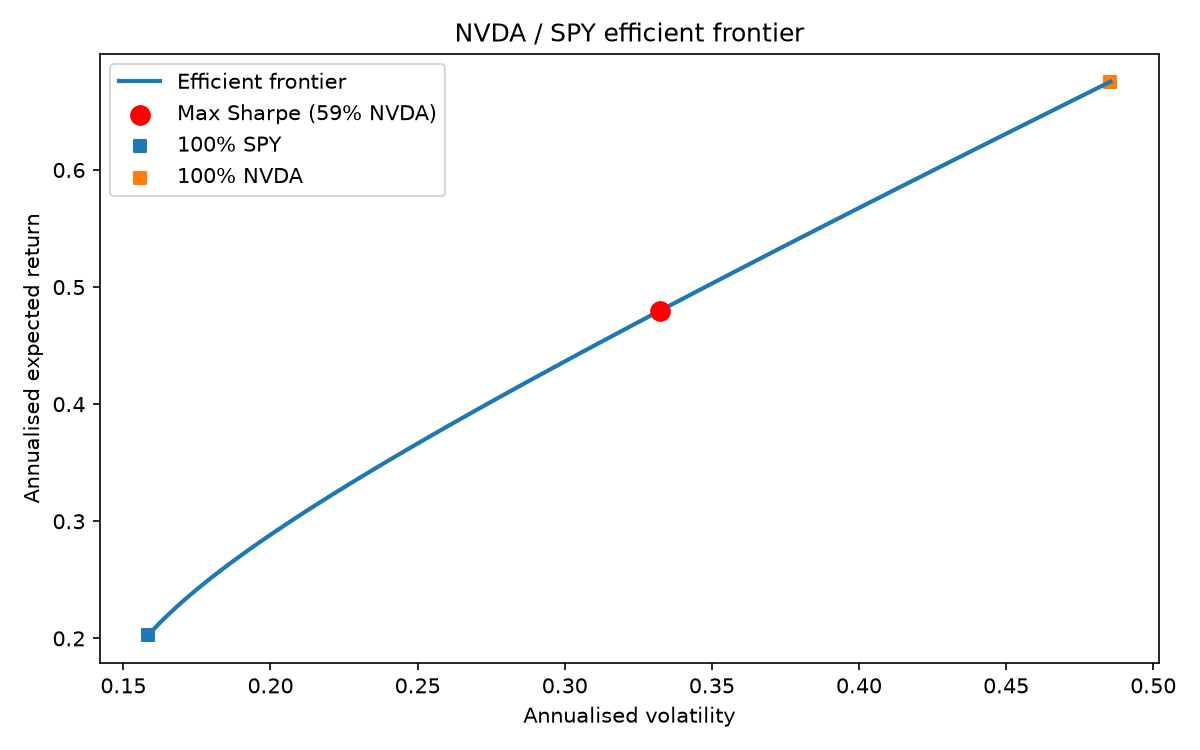
The curve shows how adding NVDA increases both expected return and volatility. The red dot is Elena's maximum Sharpe portfolio — the mix she would quote if the client cares about return per unit of risk.

See the sample efficient frontier.

Section 6 — Compare to equal weight

Question

Is 50/50 close to optimal?

Code

w_equal = np.array([0.5, 0.5])
ret_equal = w_equal @ mean_annual.values
vol_equal = np.sqrt(w_equal @ cov_annual.values @ w_equal)
sharpe_equal = (ret_equal - risk_free_annual) / vol_equal

pd.DataFrame({
    "NVDA weight": [opt_w_nvda, 0.5],
    "Expected return": [opt_return, ret_equal],
    "Volatility": [opt_vol, vol_equal],
    "Sharpe": [opt_sharpe, sharpe_equal],
}, index=["Max Sharpe", "50/50"])

What the code does

Equal weight is a common benchmark. If it is close to the optimum, the decision matters less. If it is far, optimisation adds real value — or false precision, depending on how much you trust the inputs.

Section 7 — Write Elena's summary

Add a markdown cell answering:

What NVDA weight maximises Sharpe in your sample?
How much return and volatility does that portfolio have (annualised)?
Is 100% NVDA on the frontier? Why might a client still reject it?
What could go wrong if we trust two years of historical means and covariances?

Create report/module2_frontier_summary.md (150–250 words) explaining the optimal mix to a non-technical charity trustee.

Reflection questions

Did the optimal weight surprise you?
Does plotting the frontier make diversification feel concrete?
Would you trust historical optimisation for the next five years?

Manager feedback

From: Elena Vasquez

Solid optimisation work. Remember:

Garbage in, garbage out — expected returns are the least stable input.

Constraints matter — real clients cap single-stock weight; we did not.

Sharpe is not everything — tail risk and drawdowns also matter.

Next: derivatives. Options are where the covariance matrix meets nonlinear payoffs.

— Elena

AQA Mathematics links

Quadratic expressions — portfolio variance as a weighted sum with cross-terms
Optimisation — finding a maximum on a grid
Gradients and rates — return per unit of risk

Beyond A-Level

Look up Markowitz optimisation and Black-Litterman model. Practitioners often shrink expected returns toward the market because raw historical means are noisy.

Module 3 — Derivatives

Manager email

From: Elena Vasquez
Subject: A client asked about call options on NVIDIA

We are not trading options yet, but I need you to understand the basics.

Plot payoffs at expiry for a call and a put (same strike, same underlying).

Estimate a Black-Scholes call price for one NVDA call using current inputs — no derivation required, just implement the formula with scipy.stats.norm.

Explain in plain English: what moves the price up or down?

Use NVIDIA's latest closing price from your CSV as the spot price. Assume strike = spot, 30 days to expiry, 4% risk-free rate, 40% annual volatility.

— Elena

Why this matters

Derivatives are contracts whose value depends on something else — usually a stock price. Options give the right, not the obligation, to buy (call) or sell (put) at a strike price by an expiry date.

Quants price options to manage risk, structure client payoffs, and detect when the market disagrees with a model (implied volatility).

You will not derive Black-Scholes here. You will use it — the way many junior quants start.

What you'll learn

Call and put payoff diagrams at expiry
The ingredients of Black-Scholes: spot, strike, time, rate, volatility
Implement the Black-Scholes call formula with scipy.stats.norm
Interpret how each input affects option value

Step 1 — Create the notebook

notebooks/module3_derivatives.ipynb

Section 1 — Spot price from data

Question

What is NVIDIA trading at in our sample?

Code

import pandas as pd
import numpy as np
import matplotlib.pyplot as plt
from scipy.stats import norm

nvda = pd.read_csv("../data/NVDA.csv")
nvda["Date"] = pd.to_datetime(nvda["Date"])
col = "Adj Close" if "Adj Close" in nvda.columns else "Close"
nvda = nvda.sort_values("Date")

S = nvda[col].iloc[-1]  # latest spot price
K = S                     # at-the-money strike
S, K

What the code does

S is the current stock price (spot). We set K = S so the option is at-the-money — a simple starting point. Real desks use live prices; we use the last row of our CSV.

Section 2 — Call payoff at expiry

Question

What does the holder receive at expiry for each possible stock price?

A European call pays $\max(S_T - K, 0)$ at expiry.

Code

spot_at_expiry = np.linspace(S * 0.5, S * 1.5, 200)
call_payoff = np.maximum(spot_at_expiry - K, 0)
put_payoff = np.maximum(K - spot_at_expiry, 0)

plt.figure(figsize=(8, 5))
plt.plot(spot_at_expiry, call_payoff, label="Long call")
plt.plot(spot_at_expiry, put_payoff, label="Long put")
plt.axvline(K, color="gray", linestyle="--", linewidth=0.8, label="Strike")
plt.xlabel("NVDA price at expiry")
plt.ylabel("Payoff (£ per share)")
plt.title(f"Option payoffs at expiry (K = £{K:.2f})")
plt.legend()
plt.savefig("../outputs/charts/module3_option_payoffs.png", dpi=150)
plt.show()

What the code does

Below the strike, the call is worthless — you would not exercise the right to buy above market. Above the strike, the call gains £1 for every £1 the stock rises above K.

The put is the mirror: it pays when the stock finishes below the strike.

Section 3 — Black-Scholes call price

Question

What is the option worth today, before expiry?

The Black-Scholes formula for a European call:

C = S \Phi(d_1) - K e^{-rT} \Phi(d_2)

where

d_1 = \frac{\ln(S/K) + (r + \sigma^2/2)T}{\sigma\sqrt{T}}, \quad d_2 = d_1 - \sigma\sqrt{T}

and $\Phi$ is the standard normal cumulative distribution function.

Code

T = 30 / 365       # 30 days in years
r = 0.04           # 4% annual risk-free rate
sigma = 0.40       # 40% annual volatility (Elena's assumption)

d1 = (np.log(S / K) + (r + 0.5 * sigma**2) * T) / (sigma * np.sqrt(T))
d2 = d1 - sigma * np.sqrt(T)

call_price = S * norm.cdf(d1) - K * np.exp(-r * T) * norm.cdf(d2)
call_price

What the code does

norm.cdf is $\Phi$ — the area under the standard normal curve up to a point. That probability weighting is what converts a random future stock price into a fair value today.

We assume no dividends and European exercise (only at expiry). Real NVDA options are American (exercise anytime) and pay no dividend in some periods — this is a teaching simplification.

Section 4 — Sensitivity to volatility

Question

How much does option price change if volatility changes?

Code

vols = np.linspace(0.15, 0.80, 50)
prices = []

for sig in vols:
    d1 = (np.log(S / K) + (r + 0.5 * sig**2) * T) / (sig * np.sqrt(T))
    d2 = d1 - sig * np.sqrt(T)
    c = S * norm.cdf(d1) - K * np.exp(-r * T) * norm.cdf(d2)
    prices.append(c)

plt.figure(figsize=(7, 4))
plt.plot(vols, prices)
plt.xlabel("Annual volatility (sigma)")
plt.ylabel("Call price")
plt.title("Black-Scholes call price vs volatility")
plt.savefig("../outputs/charts/module3_vol_sensitivity.png", dpi=150)
plt.show()

What the code does

Higher volatility means more chance of a big move before expiry — good for the call holder, bad for the writer. The curve rises because vega (sensitivity to vol) is positive for long calls.

Section 5 — Compare moneyness

Question

What if the strike is 10% above spot (out-of-the-money)?

Code

strikes = [S * 0.9, S, S * 1.1]
labels = ["10% ITM (K < S)", "ATM (K = S)", "10% OTM (K > S)"]

rows = []
for K_test, label in zip(strikes, labels):
    d1 = (np.log(S / K_test) + (r + 0.5 * sigma**2) * T) / (sigma * np.sqrt(T))
    d2 = d1 - sigma * np.sqrt(T)
    c = S * norm.cdf(d1) - K_test * np.exp(-r * T) * norm.cdf(d2)
    rows.append({"label": label, "strike": K_test, "call_price": c})

pd.DataFrame(rows)

What the code does

In-the-money calls (strike below spot) are worth more — they already have intrinsic value. Out-of-the-money calls are cheaper lottery tickets on a big rally.

Section 6 — Write Elena's summary

Add a markdown cell answering:

What is the Black-Scholes price for the at-the-money 30-day call?
Name three inputs that would increase the call price if all else equal.
Why is the payoff chart kinked at the strike but the Black-Scholes price smooth?
Would you expect real market option prices to match this exactly? Why not?

Create report/module3_options_note.md (200–300 words) explaining to Elena what a call option is and what her client would pay for upside exposure.

Reflection questions

Did the formula feel magical or logical once you saw the inputs?
Would you prefer pricing options or building stock portfolios?
Does volatility as a "price input" make sense given Module 1 and 2?

Manager feedback

From: Elena Vasquez

Good first pass on options. Keep these straight:

Payoff ≠ profit — you pay premium upfront; the diagram is at expiry before subtracting cost.

Model ≠ market — Black-Scholes assumes constant vol and log-normal prices. NVDA jumps.

Greeks come next — delta, gamma, vega describe sensitivities; desks live on them.

You now have stocks, portfolios, and options. Next we test strategies with more statistical discipline.

— Elena

AQA Mathematics links

Functions and graphs — piecewise linear payoffs
Exponentials and logarithms — discount factor $e^{-rT}$ , $\ln(S/K)$
Normal distribution — $\Phi$ as cumulative probability

Beyond A-Level

Look up implied volatility — the vol that makes Black-Scholes match the market price. It is often called "the wrong number in the wrong formula to get the right price."

Module 4 — Strategies

Manager email

From: Elena Vasquez
Subject: Momentum or mean reversion on NVIDIA — pick a side with evidence

Two analysts argue:

Analyst A: "NVDA trends — buy after positive 5-day returns (momentum)."

Analyst B: "NVDA snaps back — buy after negative 5-day returns (mean reversion)."

Test both rules on two years of NVDA data. Compare each to buy-and-hold using:

Total compounded return

Annualised Sharpe ratio (4% risk-free rate)

A simple t-test on daily strategy returns vs zero mean (use scipy.stats.ttest_1samp)

I want a verdict: which story fits this sample better? Could either result be luck?

— Elena

Why this matters

Quant 101 tested one moving-average rule informally. Now you compare competing hypotheses with summary statistics and a basic significance test.

Momentum and mean reversion are opposite beliefs about how prices behave after a move. Both cannot be universally true — but either might work in certain stocks or periods.

What you'll learn

Code a momentum signal from past returns
Code a mean-reversion signal from past returns
Backtest with proper signal lag (no look-ahead bias)
Compare Sharpe ratios across strategies
Run a one-sample t-test and interpret p-values cautiously

Step 1 — Create the notebook

notebooks/module4_strategies.ipynb

Section 1 — Load NVDA returns

Question

Do we have a clean return series?

Code

import pandas as pd
import numpy as np
import matplotlib.pyplot as plt
from scipy.stats import ttest_1samp

nvda = pd.read_csv("../data/NVDA.csv")
nvda["Date"] = pd.to_datetime(nvda["Date"])
col = "Adj Close" if "Adj Close" in nvda.columns else "Close"
prices = nvda.sort_values("Date")[[ "Date", col]].rename(columns={col: "price"})
prices["return"] = prices["price"].pct_change()
prices = prices.dropna().reset_index(drop=True)
prices.head()

What the code does

Same loading pattern as Quant 101 Module 3 — consistency reduces errors when Elena asks you to rerun this next quarter.

Section 2 — Past 5-day return signal

Question

Was the last week positive or negative?

Code

prices["past_5d"] = prices["price"].pct_change(5)

prices[["Date", "return", "past_5d"]].tail()

What the code does

pct_change(5) is the return over the previous five trading days (not calendar days). That is our signal input — no future data.

Section 3 — Momentum and mean-reversion signals

Question

When is each strategy invested?

Code

# Momentum: invested when past 5-day return > 0
prices["signal_mom"] = (prices["past_5d"] > 0).astype(int)

# Mean reversion: invested when past 5-day return < 0
prices["signal_mr"] = (prices["past_5d"] < 0).astype(int)

# Shift by 1 day — trade on yesterday's signal
prices["ret_mom"] = prices["return"] * prices["signal_mom"].shift(1)
prices["ret_mr"] = prices["return"] * prices["signal_mr"].shift(1)
prices["ret_bh"] = prices["return"]

prices[["Date", "signal_mom", "signal_mr", "ret_mom", "ret_mr"]].tail()

What the code does

Momentum is long when recent performance was positive — "winners keep winning."

Mean reversion is long when recent performance was negative — "losers bounce."

We multiply daily returns by yesterday's signal so we do not cheat with same-day information.

Section 4 — Cumulative performance

Question

Which strategy grew £1 the most?

Code

bt = prices.dropna(subset=["past_5d", "ret_mom", "ret_mr"]).copy()

for col in ["ret_bh", "ret_mom", "ret_mr"]:
    bt[f"cum_{col}"] = (1 + bt[col].fillna(0)).cumprod()

final = {
    "Buy and hold": bt["cum_ret_bh"].iloc[-1] - 1,
    "Momentum": bt["cum_ret_mom"].iloc[-1] - 1,
    "Mean reversion": bt["cum_ret_mr"].iloc[-1] - 1,
}
pd.Series(final)

What the code does

Compounding daily returns gives total performance over the backtest window. This is the headline number — but not the only one Elena wants.

Section 5 — Sharpe ratios

Question

Which strategy earned the best return per unit of risk?

Code

risk_free_daily = 0.04 / 252

def annualised_sharpe(daily_returns):
    excess = daily_returns - risk_free_daily
    return np.sqrt(252) * excess.mean() / excess.std()

sharpes = {
    "Buy and hold": annualised_sharpe(bt["ret_bh"]),
    "Momentum": annualised_sharpe(bt["ret_mom"].fillna(0)),
    "Mean reversion": annualised_sharpe(bt["ret_mr"].fillna(0)),
}
pd.Series(sharpes)

What the code does

Sharpe uses excess return over the risk-free rate. A strategy can beat buy-and-hold on total return but lose on Sharpe if it is much bumpier.

Days when the signal is 0, strategy return is 0 — we sit in cash. That lowers volatility but also misses upside.

Section 6 — t-test on strategy returns

Question

Is the average daily strategy return statistically different from zero?

Code

t_mom, p_mom = ttest_1samp(bt["ret_mom"].dropna(), 0)
t_mr, p_mr = ttest_1samp(bt["ret_mr"].dropna(), 0)

pd.DataFrame({
    "t-statistic": [t_mom, t_mr],
    "p-value": [p_mom, p_mr],
}, index=["Momentum", "Mean reversion"])

What the code does

ttest_1samp tests whether the mean of daily strategy returns differs from zero.

p-value small (e.g. < 0.05) suggests the mean is unlikely to be zero if returns were truly random noise — but two years of one stock is not a rigorous proof.
t-statistic sign tells you direction — positive mean excess.

Finance quants treat p-values carefully: markets are not independent coin flips.

Section 7 — Chart cumulative paths

Question

What would Elena see?

Code

plt.figure(figsize=(10, 5))
plt.plot(bt["Date"], bt["cum_ret_bh"], label="Buy and hold")
plt.plot(bt["Date"], bt["cum_ret_mom"], label="Momentum (5d)")
plt.plot(bt["Date"], bt["cum_ret_mr"], label="Mean reversion (5d)")
plt.ylabel("Growth of £1")
plt.title("NVDA: momentum vs mean reversion vs buy-and-hold")
plt.legend()
plt.savefig("../outputs/charts/module4_strategy_comparison.png", dpi=150)
plt.show()

What the code does

Visual comparison shows when each rule wins — often one strategy leads in trending periods and loses in choppy ones.

Section 8 — Verdict for Elena

Add a markdown cell answering:

Which strategy had the highest total return? The highest Sharpe?
What do the p-values suggest about momentum vs mean reversion in this sample?
Are momentum and mean reversion mutually exclusive over time — could each work in different regimes?
List three reasons the "winning" strategy might fail out-of-sample.

Create report/module4_strategy_verdict.md (250–350 words) with a clear recommendation: would Aurora deploy either rule? Why or why not?

Reflection questions

Did you hope one side would win before running the test?
Do p-values feel comforting or misleading for financial data?
Would you rather research strategies or execute them under pressure?

Manager feedback

From: Elena Vasquez

This is how desks settle arguments — with numbers, not slides.

If both p-values are high, neither story is proven — that is common.

If momentum wins in an AI rally, ask whether the rule is just "be long NVDA."

Transaction costs would hurt mean reversion more if it switches often.

Final assignment: propose your own rule. Make it simple, test it honestly, and write me a memo I could forward to a client committee.

— Elena

AQA Mathematics links

Hypothesis testing — t-test, p-values, null hypothesis
Sampling and inference — sample mean vs population
Sequences — compounding returns over time

Beyond A-Level

Look up multiple testing and data snooping. Testing many rules on the same data inflates false positives — a major reason quant funds employ strict research protocols.

Module 5 — Capstone

Manager email

From: Elena Vasquez
Subject: Your strategy — research memo for the investment committee

This is your capstone. Design one simple quantitative strategy using data you already have (NVDA, AAPL, SPY — combine them if you wish).

Requirements:

State a clear ** hypothesis** in one sentence.

Define entry and exit rules precisely — no vague language.

Backtest on your two-year sample with no look-ahead bias.

Report total return, annualised volatility, Sharpe ratio, and maximum drawdown (largest peak-to-trough fall in cumulative wealth).

Compare to buy-and-hold on your primary asset.

Write a 400–600 word memo in report/module5_capstone_memo.md for me to forward to a client committee.

Keep it simple. A clean vol-targeting rule or dual-asset rotation beats a overfit neural network you cannot explain.

Due: end of this module.

— Elena

Why this matters

Junior quants are judged on clarity as much as code. A committee memo forces you to connect hypothesis, method, results, limitations, and recommendation — the same structure as sell-side research and internal risk reviews.

This is the closest thing in the course to a first-week task on a graduate desk.

What you'll learn

Frame a testable investment hypothesis
Implement a complete backtest pipeline
Compute drawdown — a risk metric clients understand
Write a professional memo with honest limitations
Defend or reject your own idea under scrutiny

Example strategy ideas (pick one or invent your own)

Idea	Hypothesis sketch
Vol filter	Only hold NVDA when 20-day volatility is below its 60-day average
Relative strength	Hold NVDA when its 20-day return beats SPY; otherwise hold SPY
Dual MA on SPY	Use SPY trend to decide NVDA exposure (risk-on / risk-off)
Drawdown control	Cut exposure by half if NVDA falls 10% from its trailing peak

Do not copy Quant 101's 20/50 MA unchanged — extend or combine ideas.

Step 1 — Create the notebook

notebooks/module5_capstone.ipynb

Section 1 — Load all data

Question

Are NVDA, AAPL and SPY aligned?

Code

import pandas as pd
import numpy as np
import matplotlib.pyplot as plt

def load_prices(path):
    df = pd.read_csv(path)
    df["Date"] = pd.to_datetime(df["Date"])
    col = "Adj Close" if "Adj Close" in df.columns else "Close"
    df = df.sort_values("Date")
    return df[["Date", col]].rename(columns={col: "price"})

nvda = load_prices("../data/NVDA.csv")
spy = load_prices("../data/SPY.csv")
aapl = load_prices("../data/AAPL.csv")

data = nvda.merge(spy, on="Date", suffixes=("_nvda", "_spy"))
data = data.merge(aapl, on="Date")
data = data.rename(columns={"price": "price_aapl"})
data["ret_nvda"] = data["price_nvda"].pct_change()
data["ret_spy"] = data["price_spy"].pct_change()
data = data.dropna().reset_index(drop=True)
data.head()

What the code does

We keep prices and returns for all three names on shared dates. Your strategy may use only NVDA, or rotate between NVDA and SPY — align everything first.

Section 2 — Example: relative strength signal

Question

Does NVDA outperform the market over the last 20 days?

Below is one worked example. Replace with your own rules if you chose a different strategy.

Code

data["nvda_20d"] = data["price_nvda"].pct_change(20)
data["spy_20d"] = data["price_spy"].pct_change(20)

# 1 = hold NVDA, 0 = hold SPY (cash proxy)
data["signal"] = (data["nvda_20d"] > data["spy_20d"]).astype(int)
data["signal"] = data["signal"].shift(1)  # no look-ahead

data["ret_strategy"] = (
    data["signal"] * data["ret_nvda"] +
    (1 - data["signal"]) * data["ret_spy"]
)
data["ret_benchmark"] = data["ret_nvda"]  # buy-and-hold NVDA

data[["Date", "signal", "ret_strategy", "ret_benchmark"]].tail()

What the code does

When NVDA's 20-day return beats SPY's, we hold NVDA; otherwise we hold SPY as a defensive proxy. The signal is lagged one day.

If this is not your strategy, rewrite this section with your own hypothesis and rules — but keep the lag discipline.

Section 3 — Performance metrics

Question

How did the strategy perform?

Code

bt = data.dropna(subset=["ret_strategy", "ret_benchmark"]).copy()

bt["wealth_strategy"] = (1 + bt["ret_strategy"]).cumprod()
bt["wealth_benchmark"] = (1 + bt["ret_benchmark"]).cumprod()

total_ret_strat = bt["wealth_strategy"].iloc[-1] - 1
total_ret_bench = bt["wealth_benchmark"].iloc[-1] - 1

vol_strat = bt["ret_strategy"].std() * np.sqrt(252)
vol_bench = bt["ret_benchmark"].std() * np.sqrt(252)

rf_daily = 0.04 / 252
sharpe_strat = np.sqrt(252) * (bt["ret_strategy"] - rf_daily).mean() / bt["ret_strategy"].std()
sharpe_bench = np.sqrt(252) * (bt["ret_benchmark"] - rf_daily).mean() / bt["ret_benchmark"].std()

def max_drawdown(wealth):
    peak = wealth.cummax()
    dd = (wealth - peak) / peak
    return dd.min()

mdd_strat = max_drawdown(bt["wealth_strategy"])
mdd_bench = max_drawdown(bt["wealth_benchmark"])

pd.DataFrame({
    "Total return": [total_ret_strat, total_ret_bench],
    "Ann. volatility": [vol_strat, vol_bench],
    "Sharpe": [sharpe_strat, sharpe_bench],
    "Max drawdown": [mdd_strat, mdd_bench],
}, index=["Strategy", "Buy-and-hold NVDA"])

What the code does

Maximum drawdown is the worst peak-to-trough loss — clients feel drawdowns more than volatility. A strategy with high return but −50% drawdown may be unacceptable for a charity mandate.

Section 4 — Chart wealth paths

Question

Can the committee see the ride?

Code

plt.figure(figsize=(10, 5))
plt.plot(bt["Date"], bt["wealth_strategy"], label="Your strategy")
plt.plot(bt["Date"], bt["wealth_benchmark"], label="Buy-and-hold NVDA")
plt.ylabel("Growth of £1")
plt.title("Capstone backtest")
plt.legend()
plt.savefig("../outputs/charts/module5_capstone.png", dpi=150)
plt.show()

What the code does

One clear chart for the memo appendix. Mark major drawdown periods mentally — Elena will ask about them.

Section 5 — Write the investment memo

Create report/module5_capstone_memo.md with this structure:

To: Elena Vasquez, Aurora Capital
From: [Your name]
Date: [Today's date]
Subject: Proposal — [your strategy name in 5–8 words]

Executive summary (3–4 sentences) — hypothesis, verdict, recommendation.
Hypothesis — one precise sentence.
Method — data, date range, entry/exit rules, benchmark, signal lag.
Results — table or bullet list with total return, volatility, Sharpe, max drawdown; strategy vs benchmark.
Risk discussion — worst drawdown, time out of market, concentration.
Limitations — sample length, one regime, no transaction costs, no slippage, parameter choices not robustness-tested.
Recommendation — deploy, research further, or reject; one paragraph.

Write for a non-technical charity trustee who will skim the summary and read the recommendation.

A sample memo is on Worked examples.

Reflection questions

Did you trust your own strategy before seeing the backtest? After?
Which was harder — coding or writing the memo?
If Elena rejected your idea, would you be disappointed or relieved?
After Quant 101 and 201, do you want to pursue this career path?

Manager feedback

From: Elena Vasquez

I read memos in this order: summary → limitations → recommendation. Yours should survive that order.

What separates hireable juniors:

They kill strategies that only work in one chart window.

They report drawdown, not just return.

They say "I don't know" when the sample is too small.

You are still early in your journey. But you now speak the language of a quant desk: returns, covariance, options, backtests, and client memos.

If you want industry depth next, look at CQF, MFin programmes, or summer internships at the firms you researched in Quant 101.

Well done.

— Elena

AQA Mathematics links

Problem solving — translating a word hypothesis into code
Statistics — summarising and comparing distributions of returns
Communication — structured technical writing

Beyond A-Level

Look up walk-forward analysis and paper trading. The gap between a backtest and live trading is where many strategies die — costs, slippage, and regime change.

Module 6 — What You Have Learned

By the end of Quant 201, you have learned to:

build correlation and covariance matrices and run market regression for beta;
plot a two-asset efficient frontier and find the maximum Sharpe portfolio;
draw option payoffs and price a Black-Scholes call with scipy.stats.norm;
formally test momentum versus mean reversion on NVIDIA with Sharpe ratios and t-tests;
design your own strategy, backtest it with drawdown metrics, and write an investment memo for Elena.

If you enjoyed the statistics, optimisation, derivatives pricing, and evidence-based strategy work, you are thinking like a junior quant.

You completed the Aurora Capital quantitative finance track:

Quant 101 — Could I be a quant?
Quant 201 — Becoming a quant

Ready for an open brief? Continue to Quant 301 and choose your own research question.

From here, explore university courses in mathematics, finance, or computer science, seek spring weeks and internships, and keep building notebooks that measure honestly and explain clearly.